Lecture 8 - Neural Networks

Learning goals

• Explain a simple multilayer perceptron: layers, weights, bias, activation, loss, optimizer.

• Build your first neural network for a toy problem, then for small chemistry tasks.

• Train MLPRegressor and MLPClassifier step by step with diagnostics.

• Read training curves, avoid overfitting.

---

0. Setup

We will stick to a light stack so it runs everywhere.

Show code cell source

Hide code cell source

import warnings
warnings.filterwarnings("ignore")

import numpy as np
import pandas as pd
import matplotlib.pyplot as plt

from sklearn.model_selection import train_test_split
from sklearn.preprocessing import StandardScaler
from sklearn.pipeline import Pipeline
from sklearn.metrics import (mean_squared_error, mean_absolute_error, r2_score,
                             accuracy_score, precision_score, recall_score, f1_score,
                             confusion_matrix, roc_auc_score, roc_curve)
from sklearn.linear_model import LogisticRegression, LinearRegression
from sklearn.neural_network import MLPClassifier, MLPRegressor

# RDKit optional
try:
    from rdkit import Chem
    from rdkit.Chem import Descriptors, Crippen, rdMolDescriptors
except Exception:
    Chem = None

---

1. What is a neural network

Picture in words

A multilayer perceptron (MLP) takes an input vector x, multiplies by a weight matrix, adds a bias, applies a nonlinear activation like ReLU or tanh, then repeats for one or more hidden layers, and finally outputs a number (regression) or class score (classification).

Key pieces:

• Weights W and bias b set how features combine.

• Activation makes the model nonlinear so it can bend decision boundaries.

• Loss measures error. We update weights to reduce loss on the training set.

• Optimizer uses gradients to move weights a little bit each iteration (epoch).

We start tiny with a simulated dataset so we can see each piece clearly.

1.1 Generate a toy dataset and plot

rng = np.random.RandomState(0)

n = 200

# --- Base donut in 2D ---
# Outer ring
theta = rng.uniform(0, 2*np.pi, size=n)
r = 1.0 + 0.3*rng.randn(n)
X1 = np.c_[3 * r*np.cos(theta), r*np.sin(theta)]  # stretch x by 3
y1 = np.zeros(n, dtype=int)

# Inner ring
theta2 = rng.uniform(0, 2*np.pi, size=n)
r2 = 0.4 + 0.15*rng.randn(n)
X2 = np.c_[3 * r2*np.cos(theta2), r2*np.sin(theta2)]  # stretch x by 3
y2 = np.ones(n, dtype=int)

# Combine 2D
X2d = np.vstack([X1, X2])
y_toy = np.hstack([y1, y2])

angle = np.pi / 4
R = np.array([[np.cos(angle), -np.sin(angle)],
              [np.sin(angle),  np.cos(angle)]])
X2d = X2d @ R.T

f_big   = rng.normal(0, 10000.0,  size=(X2d.shape[0], 1))
f_small = rng.normal(0, 0.0001,  size=(X2d.shape[0], 1))
f_mid   = rng.normal(0, 3.0,   size=(X2d.shape[0], 1))

X_toy = np.hstack([X2d, f_big, f_small, f_mid])

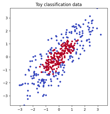
# --- Plot using the first two columns only, keep square view ---
plt.figure(figsize=(5,5))
plt.scatter(X_toy[:,0], X_toy[:,1], c=y_toy, cmap="coolwarm", s=16)

lim = max(abs(X_toy[:,0]).max(), abs(X_toy[:,1]).max())
plt.xlim(-lim, lim)
plt.ylim(-lim, lim)
plt.gca().set_aspect("equal")

plt.title("Toy classification data")
plt.show()

1.2 Split and try a linear model

Why a baseline

As in past lectures, a simple baseline tells us if a complex model is truly needed.

In scikit-learn, a pipeline is a convenient way to chain multiple steps together into a single object.
Here, our pipeline has two steps:

1. Scaler (StandardScaler): ensures each feature has zero mean and unit variance, which helps many models train more effectively.

2. Logistic Regression (LogisticRegression): the actual linear classifier that fits a straight decision boundary to the data.

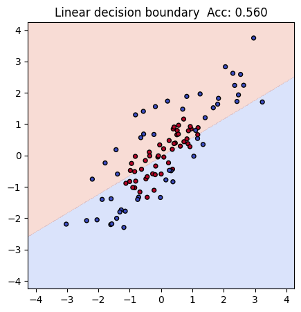
In our toy dataset, both x and y coordinates are on a similar numeric scale (roughly between -1.5 and 1.5). That means the results will look similar with or without the scaler. Still, you can see the first example has a higher acc 0.56 than the second one 0.54, and including it is good practice, because real-world datasets often have features on very different scales.

Xtr, Xte, ytr, yte = train_test_split(X_toy, y_toy, test_size=0.25, random_state=42, stratify=y_toy)

lin = Pipeline([
    ("scaler", StandardScaler()),
    ("logreg", LogisticRegression(max_iter=1000))
])
lin.fit(Xtr, ytr)

acc_lin = accuracy_score(yte, lin.predict(Xte))
print(f"Linear baseline accuracy with sacler: {acc_lin:.3f}")

Linear baseline accuracy with sacler: 0.560

By wrapping these steps in a pipeline, we can train, evaluate, and later reuse the combined process as if it were one model.

Without scaler, the result will be different in this dataset:

Xtr, Xte, ytr, yte = train_test_split(X_toy, y_toy, test_size=0.25, random_state=42, stratify=y_toy)

lin2 = LogisticRegression(max_iter=1000)
lin2.fit(Xtr, ytr)

acc_lin2 = accuracy_score(yte, lin2.predict(Xte))
print(f"Linear baseline accuracy without scaler: {acc_lin2:.3f}")

Linear baseline accuracy without scaler: 0.540

Regardless, as you can see, currently the prediction is pretty bad because linear regression itself does not handle this type of complex “donut” style dataset well due to its inherent limitation.

# Compact decision-boundary plot using only the first two features

# square limits from first two columns
lim = np.abs(np.vstack([Xtr[:, :2], Xte[:, :2]])).max()
pad = 0.5
xs = np.linspace(-lim - pad, lim + pad, 300)
ys = np.linspace(-lim - pad, lim + pad, 300)
xx, yy = np.meshgrid(xs, ys)

# build full grid (fill extra features with training means)
grid = np.c_[xx.ravel(), yy.ravel()]
if Xtr.shape[1] > 2:
    rest = np.tile(Xtr[:, 2:].mean(axis=0), (grid.shape[0], 1))
    grid = np.hstack([grid, rest])

Z = lin.predict(grid).reshape(xx.shape)

plt.figure(figsize=(5,5))
plt.contourf(xx, yy, Z, levels=2, alpha=0.25, cmap="coolwarm")
plt.scatter(Xte[:, 0], Xte[:, 1], c=yte, cmap="coolwarm", s=18, edgecolor="k")
plt.xlim(-lim - pad, lim + pad)
plt.ylim(-lim - pad, lim + pad)
plt.gca().set_aspect("equal", adjustable="box")
plt.title(f"Linear decision boundary  Acc: {acc_lin:.3f}")
plt.show()

1.3 Build a small MLP step by step

Now let’s see if we can solve this classification challenge with simple and shallow neural network.

We will build a MLP classifier by adding one hidden layer with 8 units and ReLU activation. Before we start to do it, we will first look at key concepts:

A multilayer perceptron (MLP) stacks simple building blocks:

• Linear layer: multiply by weights and add a bias. Example: z = X @ W + b

• Activation: bend the space so a straight line can become a curve. Common choices:

  • ReLU: max(0, z)

  • Tanh: squashes to [-1, 1]

  • Sigmoid: squashes to [0, 1] and is often used at the output for probability

• Loss: tells us how wrong we are. For classification we use cross entropy

• Optimizer: updates weights to reduce loss. Scikit-learn’s MLP uses SGD variants under the hood

Why ReLU

• It is simple, fast, and avoids the flat gradients that slow learning with sigmoid on hidden layers

• Many ReLU units stacked together can carve a curved boundary that a linear model cannot

Below we first look at the shapes of common activations, then we build a small MLP and read its learned shapes.

Show code cell source

Hide code cell source

# Mini gallery of activation functions in three panels
x = np.linspace(-4, 4, 400)

def relu(z):     return np.maximum(0, z)
def sigmoid(z):  return 1 / (1 + np.exp(-z))
def tanh_act(z): return np.tanh(z)

fig, axes = plt.subplots(1, 3, figsize=(12,3))

axes[0].plot(x, relu(x))
axes[0].set_title("ReLU")
axes[0].grid(alpha=0.3)

axes[1].plot(x, sigmoid(x))
axes[1].set_title("Sigmoid")
axes[1].grid(alpha=0.3)

axes[2].plot(x, tanh_act(x))
axes[2].set_title("Tanh")
axes[2].grid(alpha=0.3)

for ax in axes:
    ax.set_xlabel("z")
    ax.set_ylabel("activation(z)")

plt.tight_layout()
plt.show()

To keep it simple, imagine we have just one input \(x\), two hidden ReLU units, and one sigmoid output.

Note

Steps:

1. Hidden pre-activations
   $\( z^{(1)}_1 = w^{(1)}_{1}\,x + b^{(1)}_{1}, \quad z^{(1)}_2 = w^{(1)}_{2}\,x + b^{(1)}_{2} \)$

2. Hidden activations (apply ReLU)
   $\( h_1 = \max(0, z^{(1)}_1), \quad h_2 = \max(0, z^{(1)}_2) \)$

3. Output score and probability
   $\( z^{(2)} = v_{1} h_1 + v_{2} h_2 + b^{(2)}, \quad \hat{p} = \sigma(z^{(2)}) = \frac{1}{1 + e^{-z^{(2)}}} \)$

During training, the model learns weights \(w^{(1)}_{1}, w^{(1)}_{2}, v_1, v_2\) and biases \(b^{(1)}_{1}, b^{(1)}_{2}, b^{(2)}\) to minimize classification error.

---

Let’s look at one example with numbers so it’s easier to understand:

Suppose:

• Input: \(x = 0.5\)

• Hidden weights and biases:
  \(w^{(1)}_{1} = 2.0,\; b^{(1)}_{1} = -0.6\)
  \(w^{(1)}_{2} = -1.0,\; b^{(1)}_{2} = 0.2\)

• Output weights and bias:
  \(v_1 = 1.0,\; v_2 = -2.0,\; b^{(2)} = 0.1\)

Step 1. Hidden pre-activations
$\( z^{(1)}_1 = 2.0 \cdot 0.5 + (-0.6) = 0.4 \)\( \)\( z^{(1)}_2 = -1.0 \cdot 0.5 + 0.2 = -0.3 \)$

Step 2. Hidden activations (ReLU)
$\( h_1 = \max(0, 0.4) = 0.4 \)\( \)\( h_2 = \max(0, -0.3) = 0 \)$

Step 3. Output
$\( z^{(2)} = 1.0 \cdot 0.4 + (-2.0) \cdot 0 + 0.1 = 0.5 \)\( \)\( \hat{p} = \sigma(0.5) = \frac{1}{1+e^{-0.5}} \approx 0.62 \)$

So with this set of weights, input \(x=0.5\) is classified with probability \(\hat{p} \approx 0.62\) for class 1.

Show code cell source

Hide code cell source

from matplotlib.patches import Circle, FancyArrowPatch

# --- example parameters ---
x = 0.5
w1, b1 = 2.0, -0.6   # hidden 1
w2, b2 = -1.0, 0.2   # hidden 2
v1, v2, b_out = 1.0, -2.0, 0.1  # output

# --- forward pass ---
z1 = w1*x + b1
z2 = w2*x + b2
h1, h2 = relu(z1), relu(z2)
z_out = v1*h1 + v2*h2 + b_out
p_hat = sigmoid(z_out)

# --- node positions ---
nodes = {
    "x": (0, 0),
    "h1": (2, 1),
    "h2": (2, -1),
    "y": (4, 0),
}

def draw_node(ax, name, label, value=None, radius=0.35):
    cx, cy = nodes[name]
    c = Circle((cx, cy), radius, fc="white", ec="k", lw=1.2)
    ax.add_patch(c)
    ax.text(cx, cy, label, ha="center", va="center", fontsize=11)
    if value is not None:
        ax.text(cx, cy - radius - 0.15, f"{value:.2f}",
                ha="center", va="top", fontsize=9, color="blue")

def draw_arrow(ax, a, b, lbl_top, lbl_bottom, radius=0.35, y_offset=0.45):
    (x1, y1), (x2, y2) = nodes[a], nodes[b]
    dx, dy = x2 - x1, y2 - y1
    dist = np.sqrt(dx**2 + dy**2)
    shrink = radius / dist
    start = (x1 + dx*shrink, y1 + dy*shrink)
    end   = (x2 - dx*shrink, y2 - dy*shrink)
    arrow = FancyArrowPatch(start, end, arrowstyle="-|>", mutation_scale=12, lw=1.0)
    ax.add_patch(arrow)
    xm, ym = (start[0]+end[0])/2, (start[1]+end[1])/2
    ax.text(xm, ym+y_offset, lbl_top, fontsize=8, ha="center")
    ax.text(xm, ym+y_offset-0.3, lbl_bottom, fontsize=8, ha="center")

# --- make plot ---
fig, ax = plt.subplots(figsize=(9,5))

# generic formulas at top (just linear + ReLU now)
ax.text(2, 2.3, r"$z = w \cdot x + b$", fontsize=12, ha="center")
ax.text(2, 1.9, r"$h = \max(0, z)$", fontsize=12, ha="center")

# nodes with values
draw_node(ax, "x", "$x$", x)
draw_node(ax, "h1", "$h_1$", h1)
draw_node(ax, "h2", "$h_2$", h2)
draw_node(ax, "y", "$\\hat{p}$", p_hat)

# arrows input→hidden (weights and biases on two lines, moved up a bit)
draw_arrow(ax, "x", "h1", f"$w_1={w1}$", f"$b_1={b1}$", y_offset=0.55)
draw_arrow(ax, "x", "h2", f"$w_2={w2}$", f"$b_2={b2}$", y_offset=0.55)

# arrows hidden→output (bias shown near output node)
draw_arrow(ax, "h1", "y", f"$v_1={v1}$", "", y_offset=0.45)
draw_arrow(ax, "h2", "y", f"$v_2={v2}$", "", y_offset=0.45)
ax.text(nodes["y"][0]+0.6, nodes["y"][1]+0.25, f"$b={b_out}$", fontsize=9)

ax.set_xlim(-1, 7)
ax.set_ylim(-2.5, 2.5)
ax.axis("off")
ax.set_title("1 → 2 → 1 MLP with forward pass values", pad=15)

# side text with detailed calculations
text = (
    f"Input: $x={x}$\n\n"
    f"$z_1 = {w1}*{x}+({b1}) = {z1:.2f}$ → $h_1 = {h1:.2f}$\n"
    f"$z_2 = {w2}*{x}+({b2}) = {z2:.2f}$ → $h_2 = {h2:.2f}$\n\n"
    f"$z = {v1}*{h1}+{v2}*{h2}+({b_out}) = {z_out:.2f}$\n"
    f"$\\hat p = \\sigma(z) = {p_hat:.2f}$"
)
ax.text(6.2, 1.5, text, fontsize=10, va="top")

plt.show()

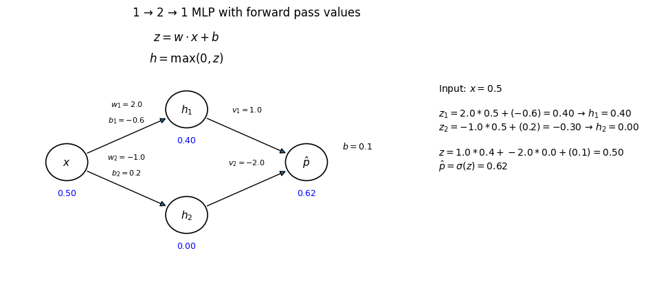
Note that in above example we already have a set of paramters so the calculation can be demonstrated.

In a real neural network, the weights \(w\) and biases \(b\) are not chosen by hand.

So, where do these numbers come from?

Try to recall what happens in linear regression.
In that case, you can compute the exact formulas for \(w\) and \(b\) by hand using sums and algebra or use lin.fit(Xtr, ytr) to get your trained function.

In a neural network, you usually don’t solve directly with formulas. Instead, you:

1. Initialize \(w\) and \(b\) randomly.

2. Adjust them step by step so that the loss (for example, mean squared error or cross-entropy) becomes smaller.

3. Run the next iteration with the updated weights, check the loss again, and adjust \(w\) and \(b\) further to aim for an even smaller loss.

4. After many updates, the parameters \(w\) and \(b\) converge to useful values — often close to what you would get from regression formulas in simple cases.

Because this process is iterative, the real learned numbers can look irregular, like \(w=0.483\) or \(b=-1.273\).
For teaching, we instead pick round numbers so it’s easier to see the flow of calculations by hand.

mlp = Pipeline([
    ("scaler", StandardScaler()),
    ("clf", MLPClassifier(hidden_layer_sizes=(8,),
                          activation="relu",
                          learning_rate_init=0.05,
                          alpha=1e-4,            # L2 penalty
                          max_iter=500,
                          random_state=0))
])
mlp

Pipeline(steps=[('scaler', StandardScaler()),
                ('clf',
                 MLPClassifier(hidden_layer_sizes=(8,), learning_rate_init=0.05,
                               max_iter=500, random_state=0))])

In a Jupyter environment, please rerun this cell to show the HTML representation or trust the notebook.
On GitHub, the HTML representation is unable to render, please try loading this page with nbviewer.org.

Fit and evaluate.

mlp.fit(Xtr, ytr)
acc_mlp = accuracy_score(yte, mlp.predict(Xte))
print(f"MLP accuracy: {acc_mlp:.3f}")

MLP accuracy: 0.890

Compared with linear regression (baseline accuracy: 0.560), we now get an MLP accuracy: 0.870, which is much higher!

1.5 Analyzing the MLP models

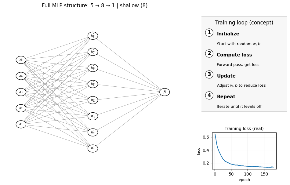
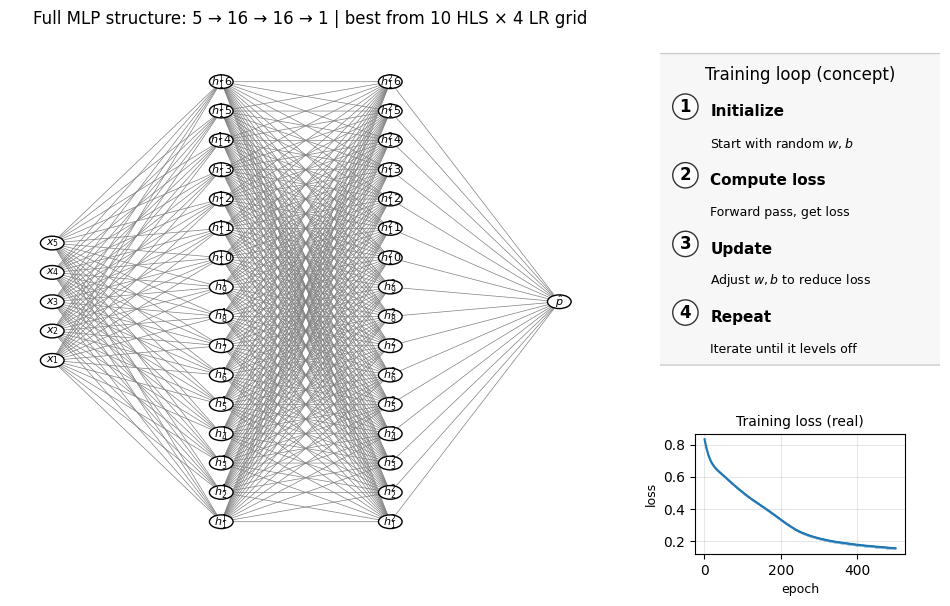
Now let’s look at the plot below to see the structure of the MLP model we built.

Remember, we have 5 input x features. In the earlier plot we only showed the first two (X–Y) for visualization, but each point actually comes from all 5 features — that 2D scatter is just a projection. Think back to the earlier lecture where a molecule could be represented by multiple features such as MolWt, LogP, etc. In the same way, here all 5 features are connected to the hidden layer (with 5 units in this example).

Show code cell source

Hide code cell source

from matplotlib.patches import Circle, FancyArrowPatch, FancyBboxPatch
def summarize_mlp(mlp_pipeline):
    clf = mlp_pipeline.named_steps["clf"]
    hidden = clf.hidden_layer_sizes if isinstance(clf.hidden_layer_sizes, tuple) else (clf.hidden_layer_sizes,)
    print("Number of layers (including input and output):", clf.n_layers_)
    print("Hidden layer sizes:", hidden)
    print("coefs_ length (weight matrices between layers):", len(clf.coefs_))
    for i, (W, b) in enumerate(zip(clf.coefs_, clf.intercepts_), start=1):
        print(f"Layer {i} weight shape:", W.shape, "  bias shape:", b.shape)

def draw_full_mlp_structure(mlp_pipeline, Xtr, title_suffix=""):
    import numpy as np
    import matplotlib.pyplot as plt
    from matplotlib.patches import Circle, FancyArrowPatch, FancyBboxPatch

    clf = mlp_pipeline.named_steps["clf"]
    n_inputs = Xtr.shape[1]
    hidden = clf.hidden_layer_sizes if isinstance(clf.hidden_layer_sizes, tuple) else (clf.hidden_layer_sizes,)
    sizes = [n_inputs] + list(hidden) + [1]

    x_spacing, y_spacing = 2.0, 0.6
    nodes = {}
    for L, width in enumerate(sizes):
        x = L * x_spacing
        ys = [(i - (width-1)/2)*y_spacing for i in range(width)]
        for i, y in enumerate(ys):
            nodes[(L, i)] = (x, y)

    fig = plt.figure(figsize=(10,6))
    ax = fig.add_axes([0.05, 0.06, 0.60, 0.88])
    rx = fig.add_axes([0.70, 0.06, 0.28, 0.88])
    ax.axis("off"); rx.axis("off")

    # Connections
    for L in range(len(sizes)-1):
        for i in range(sizes[L]):
            for j in range(sizes[L+1]):
                start, end = nodes[(L,i)], nodes[(L+1,j)]
                ax.add_patch(FancyArrowPatch(start, end, arrowstyle="-", lw=0.5, color="gray",
                                             connectionstyle="arc3,rad=0"))

    # Nodes
    R = 0.14
    for (L,i), (cx,cy) in nodes.items():
        c = Circle((cx,cy), R, fc="white", ec="k", lw=1)
        ax.add_patch(c)
        if L == 0:
            ax.text(cx, cy, f"$x_{i+1}$", ha="center", va="center", fontsize=8)
        elif L == len(sizes)-1:
            ax.text(cx, cy, "$\\hat p$", ha="center", va="center", fontsize=8)
        else:
            ax.text(cx, cy, f"$h^{L}_{i+1}$", ha="center", va="center", fontsize=8)

    arch = " → ".join([str(s) for s in sizes])
    ax.set_title(f"Full MLP structure: {arch}{(' | ' + title_suffix) if title_suffix else ''}", pad=10)

    # Right panel: steps box
    box = FancyBboxPatch((0.00, 0.40), 1.00, 0.55,
                         boxstyle="round,pad=0.02,rounding_size=0.02",
                         fc="#f7f7f7", ec="#cccccc")
    rx.add_patch(box)
    rx.text(0.50, 0.92, "Training loop (concept)", ha="center", fontsize=12)

    steps = [
        ("1", "Initialize", "Start with random $w, b$"),
        ("2", "Compute loss", "Forward pass, get loss"),
        ("3", "Update", "Adjust $w, b$ to reduce loss"),
        ("4", "Repeat", "Iterate until it levels off"),
    ]
    y0 = 0.86
    for idx, (num, title, line) in enumerate(steps):
        y = y0 - idx*0.13
        rx.text(0.07, y, num, fontsize=12, weight="bold",
                bbox=dict(boxstyle="circle,pad=0.22", fc="#ffffff", ec="#333333"))
        rx.text(0.18, y, title, fontsize=11, weight="bold", va="center")
        rx.text(0.18, y-0.06, line, fontsize=9, va="center")

    # Real loss curve (fallback to mock if unavailable)
    axc = fig.add_axes([0.735, 0.08, 0.21, 0.20])
    loss_curve = getattr(clf, "loss_curve_", None)
    if loss_curve and len(loss_curve) > 0:
        epochs = np.arange(1, len(loss_curve)+1)
        axc.plot(epochs, loss_curve, marker="o", markersize=0.1)
        axc.set_title("Training loss (real)", fontsize=10)
    else:
        print("Mock loss curve only")
        epochs = np.array([0, 1, 2, 5, 20, 50, 100])
        loss =   np.array([1.2, 0.95, 0.78, 0.55, 0.36, 0.31, 0.30])
        axc.plot(epochs, loss, marker="o", markersize=1)
        axc.set_title("Training loss (mock)", fontsize=1)

    axc.set_xlabel("epoch", fontsize=9)
    axc.set_ylabel("loss", fontsize=9)
    axc.grid(alpha=0.3)

    ax.set_xlim(-0.5, x_spacing*(len(sizes)-1)+0.6)
    ax.set_ylim(-max(sizes)/2*y_spacing-0.6, max(sizes)/2*y_spacing+0.6)
    plt.show()

mlp_shallow = mlp 
summarize_mlp(mlp_shallow); draw_full_mlp_structure(mlp_shallow, Xtr, "shallow (8)")

Number of layers (including input and output): 3
Hidden layer sizes: (8,)
coefs_ length (weight matrices between layers): 2
Layer 1 weight shape: (5, 8)   bias shape: (8,)
Layer 2 weight shape: (8, 1)   bias shape: (1,)

Does it mean that the more complex the MLP, the better results we can? Well, not necessaily. Look at the examlple below, where instead of just 1 layer we have 3 hidden layers (4 layers in total including the final output layer):

mlp_deep = Pipeline([
    ("scaler", StandardScaler()),
    ("clf", MLPClassifier(hidden_layer_sizes=(8,5,3),
                          activation="relu",
                          learning_rate_init=0.05,
                          max_iter=500,
                          random_state=0))
])

mlp_deep.fit(Xtr, ytr)
acc_mlp_deep = accuracy_score(yte, mlp_deep.predict(Xte))
print(f"MLP_deep accuracy: {acc_mlp_deep:.3f}")
summarize_mlp(mlp_deep);    draw_full_mlp_structure(mlp_deep, Xtr, "deep (8,5,3)")

MLP_deep accuracy: 0.760
Number of layers (including input and output): 5
Hidden layer sizes: (8, 5, 3)
coefs_ length (weight matrices between layers): 4
Layer 1 weight shape: (5, 8)   bias shape: (8,)
Layer 2 weight shape: (8, 5)   bias shape: (5,)
Layer 3 weight shape: (5, 3)   bias shape: (3,)
Layer 4 weight shape: (3, 1)   bias shape: (1,)

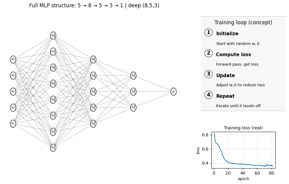
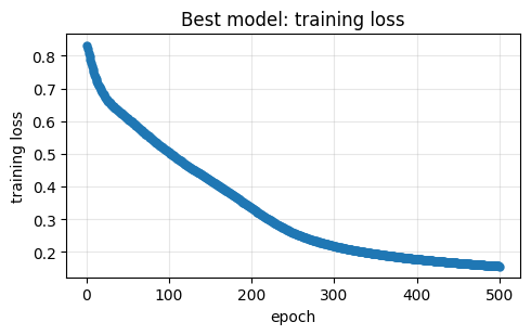
The accuray actually drops down! If you look at the loss function above, it’s also worse than the simple 5-5-1 shallow MLP we showed as the first example. Just recall the decision tree lecture we had before, the lesson is that you can’t just make super complex model to increase the accuracy because the overfitting issue will come at a certain point.

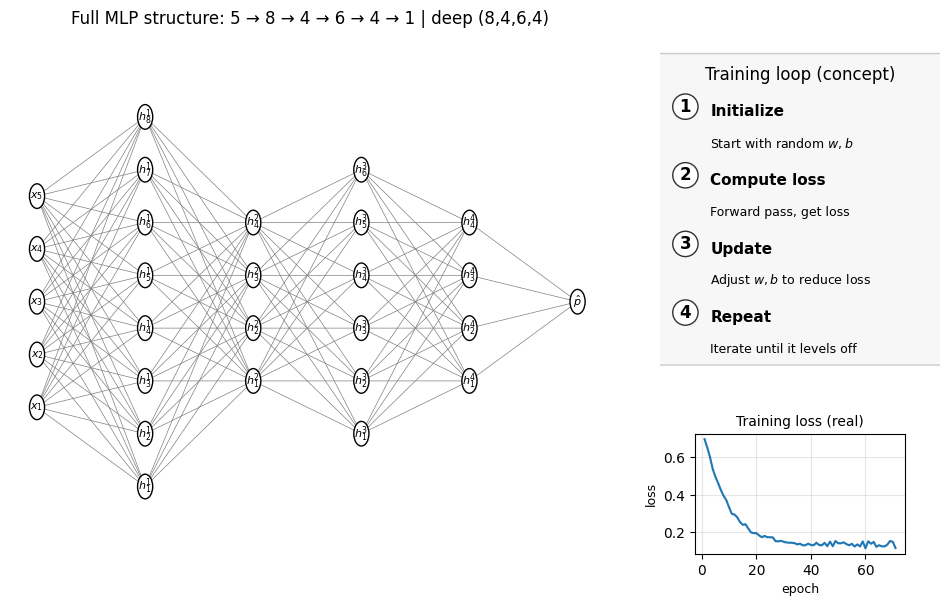
But it doesn’t necessarily mean we shouldn’t do it. Below is another case and we actually achieve a higher performance.

mlp_deep_2 = Pipeline([
    ("scaler", StandardScaler()),
    ("clf", MLPClassifier(hidden_layer_sizes=(8,4,6,4),
                          activation="relu",
                          learning_rate_init=0.05,
                          max_iter=500,
                          random_state=0))
])

mlp_deep_2.fit(Xtr, ytr)
acc_mlp_deep_2 = accuracy_score(yte, mlp_deep_2.predict(Xte))
print(f"MLP_deep_2 accuracy: {acc_mlp_deep_2:.3f}")
summarize_mlp(mlp_deep_2);    draw_full_mlp_structure(mlp_deep_2, Xtr, "deep (8,4,6,4)")

MLP_deep_2 accuracy: 0.870
Number of layers (including input and output): 6
Hidden layer sizes: (8, 4, 6, 4)
coefs_ length (weight matrices between layers): 5
Layer 1 weight shape: (5, 8)   bias shape: (8,)
Layer 2 weight shape: (8, 4)   bias shape: (4,)
Layer 3 weight shape: (4, 6)   bias shape: (6,)
Layer 4 weight shape: (6, 4)   bias shape: (4,)
Layer 5 weight shape: (4, 1)   bias shape: (1,)

1.6 Decision surface

We can plot a decision surface to see the boundary and compare all these three models.

import numpy as np
import matplotlib.pyplot as plt

# square limits from the first two columns
lim = np.abs(np.vstack([Xtr[:, :2], Xte[:, :2]])).max()
pad = 0.5
xs = np.linspace(-lim - pad, lim + pad, 300)
ys = np.linspace(-lim - pad, lim + pad, 300)
xx, yy = np.meshgrid(xs, ys)

# 2D grid for the first two features
grid2 = np.c_[xx.ravel(), yy.ravel()]

# fill the remaining features with training means (raw space)
if Xtr.shape[1] > 2:
    rest_means = Xtr[:, 2:].mean(axis=0)                 # shape (3,)
    rest = np.tile(rest_means, (grid2.shape[0], 1))      # shape (N, 3)
    grid_full = np.hstack([grid2, rest])                 # shape (N, 5)
else:
    grid_full = grid2

# probabilities for both models
zz_shallow = mlp.predict_proba(grid_full)[:, 1].reshape(xx.shape)
zz_deep    = mlp_deep.predict_proba(grid_full)[:, 1].reshape(xx.shape)
zz_deep_2  = mlp_deep_2.predict_proba(grid_full)[:, 1].reshape(xx.shape)

# plot side by side
fig, axes = plt.subplots(1, 3, figsize=(12,5), sharex=True, sharey=True)

for ax, zz, title in zip(
    axes,
    [zz_shallow, zz_deep, zz_deep_2],
    ["Shallow MLP (5 hidden)", "Deep MLP (8,5,3 hidden)", "Deep MLP (8, 4, 6, 4)"]
):
    cs = ax.contourf(xx, yy, zz, levels=20, alpha=0.4, cmap="coolwarm")  # 50% transparency
    ax.scatter(Xtr[:,0], Xtr[:,1], c=ytr, cmap="coolwarm", s=3,  alpha=0.7, label="train")
    ax.scatter(Xte[:,0], Xte[:,1], c=yte, cmap="coolwarm", s=3, marker="^", label="test")
    ax.set_aspect("equal", adjustable="box")
    ax.set_title(title)

fig.colorbar(cs, ax=axes, label="P(class=1)")
axes[0].legend(loc="lower right")
plt.show()

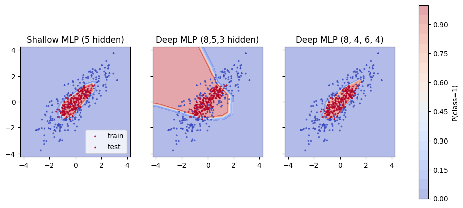
Color near 0 is class 0 and near 1 is class 1. A curved boundary shows that the hidden layer and activation created a nonlinear rule.

⏰ Exercises 1

1. Change hidden_layer_sizes=(16,) then (16,8) and compare test accuracy.

2. Switch activation from "relu" to "tanh" and rerun. Which works better here and why might that be?

3. Change learning_rate_init to 0.005 then 0.2. Watch whether the model converges. If it stalls, raise max_iter.

4. Remove the scaler from the pipeline and fit again. Record the accuracy. What changed?

1.7 Hyperparamter tuning

As we see in previous lectures, we can use cross-validation to search for the best hyperparamters. In the MLP example below, to demonstrate this idea, we can try different layer choice and learning rate. But keep in mind that there are multiple hyperparameters we can also tune. To make the demo simple we just fix most of them.

Below code will take around 2 minutes to complete, since it’s alreay 10 x 4 = 40 choices of hyperparamters.

Show code cell source

Hide code cell source

from sklearn.model_selection import GridSearchCV, StratifiedKFold
from sklearn.metrics import accuracy_score


def make_layer_choices(n_choices=20, min_layers=2, max_layers=5,
                       min_units=4, max_units=32, step=4, seed=0):
    rng = np.random.RandomState(seed)
    all_units = list(range(min_units, max_units + 1, step))

    choices = set()
    # Handful of sensible fixed patterns to ensure variety
    fixed = [
        (6,6), (6,3), (8,4),
        (8,8,4), (8,6,3), (16,8,4),
        (5,8,4,2), (8,6,6,3),
        (8,3,6,6,3), (5,8,8,6,3)
    ]
    for tpl in fixed:
        if min_layers <= len(tpl) <= max_layers:
            choices.add(tpl)
            if len(choices) == n_choices:
                return list(choices)

    # Randomly generate more until we hit n_choices
    while len(choices) < n_choices:
        L = rng.randint(min_layers, max_layers + 1)
        # Start wider, then non-increasing to keep shapes reasonable
        first = rng.choice(all_units)
        units = [first]
        for _ in range(L - 1):
            allowed = [u for u in all_units if u <= units[-1]]
            units.append(int(rng.choice(allowed)))
        choices.add(tuple(units))
    return list(choices)

def run_mlp_grid_search(Xtr, ytr, Xte, yte, layer_choices=None, lr_choices=None):
    if layer_choices is None:
        layer_choices = make_layer_choices(n_choices=20, seed=0)
    if lr_choices is None:
        lr_choices = [0.001, 0.01, 0.02, 0.05]

    base_mlp = Pipeline([
        ("scaler", StandardScaler()),
        ("clf", MLPClassifier(
            activation="relu",
            solver="adam",
            early_stopping=False, # keep early_stopping off to match direct fits, will take less time to run if turn on
            max_iter=500,
            random_state=0
        ))
    ])

    param_grid = {
        "clf__hidden_layer_sizes": layer_choices,
        "clf__learning_rate_init": lr_choices,
    }

    cv = StratifiedKFold(n_splits=5, shuffle=True, random_state=0)

    gs = GridSearchCV(
        estimator=base_mlp,
        param_grid=param_grid,
        scoring="accuracy",
        n_jobs=-1,
        cv=cv,
        refit=True,
        verbose=1
    )

    gs.fit(Xtr, ytr)

    best_pipe = gs.best_estimator_
    best_params = gs.best_params_
    acc_train = accuracy_score(ytr, best_pipe.predict(Xtr))
    acc_test  = accuracy_score(yte, best_pipe.predict(Xte))

    # Build a tidy results DataFrame
    cols = ["mean_test_score", "std_test_score", "rank_test_score"]
    df = pd.DataFrame({
        "hidden_layer_sizes": [p["clf__hidden_layer_sizes"] for p in gs.cv_results_["params"]],
        "learning_rate_init": [p["clf__learning_rate_init"] for p in gs.cv_results_["params"]],
        "mean_test_score": gs.cv_results_["mean_test_score"],
        "std_test_score": gs.cv_results_["std_test_score"],
        "rank_test_score": gs.cv_results_["rank_test_score"],
    }).sort_values("mean_test_score", ascending=False).reset_index(drop=True)

    print("\nBest CV accuracy:", f"{gs.best_score_:.3f}")
    print("Best params:", best_params)
    print("Train accuracy (refit best):", f"{acc_train:.3f}")
    print("Test  accuracy (refit best):", f"{acc_test:.3f}")
    display(df.head(10))  # top 10; remove or change to show all
    return best_pipe, df

# Run the search
layer_choices = make_layer_choices(n_choices=20, seed=0)  # 2–5 layers, 20 combos
best_pipe, results_df = run_mlp_grid_search(Xtr, ytr, Xte, yte,
                                            layer_choices=layer_choices,
                                            lr_choices=[0.001, 0.01, 0.02, 0.05])

# Optional: diagram and loss curve for the best model
summarize_mlp(best_pipe)
draw_full_mlp_structure(best_pipe, Xtr, "best from 10 HLS × 4 LR grid")

best_clf = best_pipe.named_steps["clf"]
if hasattr(best_clf, "loss_curve_") and len(best_clf.loss_curve_) > 0:
    epochs = np.arange(1, len(best_clf.loss_curve_) + 1)
    plt.figure(figsize=(5,3.2))
    plt.plot(epochs, best_clf.loss_curve_, marker="o", markersize=5, linewidth=1.5)
    plt.xlabel("epoch"); plt.ylabel("training loss")
    plt.title("Best model: training loss")
    plt.grid(alpha=0.3)
    plt.tight_layout()
    plt.show()

Fitting 5 folds for each of 80 candidates, totalling 400 fits

Best CV accuracy: 0.890
Best params: {'clf__hidden_layer_sizes': (np.int64(16), 16), 'clf__learning_rate_init': 0.001}
Train accuracy (refit best): 0.953
Test  accuracy (refit best): 0.890

	hidden_layer_sizes	learning_rate_init	mean_test_score	std_test_score	rank_test_score
0	(16, 16)	0.001	0.890000	0.027080	1
1	(8, 6, 3)	0.050	0.886667	0.038586	2
2	(24, 4, 4, 4, 4)	0.020	0.880000	0.012472	3
3	(16, 16)	0.050	0.876667	0.034319	4
4	(32, 24)	0.001	0.876667	0.037417	4
5	(12, 8)	0.010	0.876667	0.030912	4
6	(32, 28)	0.001	0.873333	0.038873	7
7	(8, 6, 3)	0.010	0.873333	0.024944	7
8	(8, 6, 3)	0.020	0.870000	0.019437	9
9	(16, 8, 4)	0.001	0.866667	0.027889	10

Number of layers (including input and output): 4
Hidden layer sizes: (np.int64(16), 16)
coefs_ length (weight matrices between layers): 3
Layer 1 weight shape: (5, 16)   bias shape: (16,)
Layer 2 weight shape: (16, 16)   bias shape: (16,)
Layer 3 weight shape: (16, 1)   bias shape: (1,)

---

2. Neural nets for chemical property prediction

We reuse the same CSV from earlier lectures and compute four quick descriptors.

url = "https://raw.githubusercontent.com/zzhenglab/ai4chem/main/book/_data/C_H_oxidation_dataset.csv"
df_raw = pd.read_csv(url)
df_raw.head(3)

	Compound Name	CAS	SMILES	Solubility_mol_per_L	pKa	Toxicity	Melting Point	Reactivity	Oxidation Site
0	3,4-dihydro-1H-isochromene	493-05-0	c1ccc2c(c1)CCOC2	0.103906	5.80	non_toxic	65.8	1	8,10
1	9H-fluorene	86-73-7	c1ccc2c(c1)Cc1ccccc1-2	0.010460	5.82	toxic	90.0	1	7
2	1,2,3,4-tetrahydronaphthalene	119-64-2	c1ccc2c(c1)CCCC2	0.020589	5.74	toxic	69.4	1	7,10

def calc_desc(smiles):
    if Chem is None:
        return pd.Series({"MolWt": np.nan, "LogP": np.nan, "TPSA": np.nan, "NumRings": np.nan})
    m = Chem.MolFromSmiles(smiles)
    if m is None:
        return pd.Series({"MolWt": np.nan, "LogP": np.nan, "TPSA": np.nan, "NumRings": np.nan})
    return pd.Series({
        "MolWt": Descriptors.MolWt(m),
        "LogP": Crippen.MolLogP(m),
        "TPSA": rdMolDescriptors.CalcTPSA(m),
        "NumRings": rdMolDescriptors.CalcNumRings(m)
    })

desc = df_raw["SMILES"].apply(calc_desc)
df = pd.concat([df_raw, desc], axis=1)
df[["Compound Name","SMILES","MolWt","LogP","TPSA","NumRings","Melting Point","Solubility_mol_per_L","Toxicity"]].head()

	Compound Name	SMILES	MolWt	LogP	TPSA	NumRings	Melting Point	Solubility_mol_per_L	Toxicity
0	3,4-dihydro-1H-isochromene	c1ccc2c(c1)CCOC2	134.178	1.7593	9.23	2.0	65.8	0.103906	non_toxic
1	9H-fluorene	c1ccc2c(c1)Cc1ccccc1-2	166.223	3.2578	0.00	3.0	90.0	0.010460	toxic
2	1,2,3,4-tetrahydronaphthalene	c1ccc2c(c1)CCCC2	132.206	2.5654	0.00	2.0	69.4	0.020589	toxic
3	ethylbenzene	CCc1ccccc1	106.168	2.2490	0.00	1.0	65.0	0.048107	non_toxic
4	cyclohexene	C1=CCCCC1	82.146	2.1166	0.00	1.0	96.4	0.060688	non_toxic

Reminder

We used these same descriptors in Lectures 5 to 7. They form a compact input vector for both regression and classification.

Neural nets are sensitive to feature scales. Always standardize inputs.

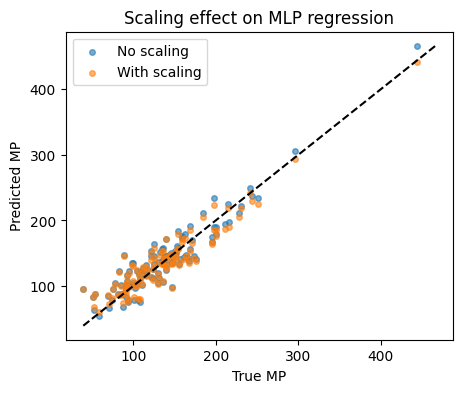
We will show MLP performance with and without StandardScaler on a quick regression target.

2.1 Target choice: melting point

df_reg = df[["MolWt","LogP","TPSA","NumRings","Melting Point"]].dropna()
X = df_reg[["MolWt","LogP","TPSA","NumRings"]].values
y = df_reg["Melting Point"].values

X_train, X_test, y_train, y_test = train_test_split(X, y, test_size=0.2, random_state=42)
X_train.shape, X_test.shape

((460, 4), (115, 4))

MLP without scaling:

mlp_raw = MLPRegressor(hidden_layer_sizes=(64,32),
                       activation="relu",
                       learning_rate_init=0.01,
                       alpha=1e-4,
                       max_iter=1000,
                       random_state=0)
mlp_raw.fit(X_train, y_train)
y_pred_raw = mlp_raw.predict(X_test)
print(f"R2 no scaling: {r2_score(y_test, y_pred_raw):.3f}")

R2 no scaling: 0.867

MLP with scaling:

mlp_scaled = Pipeline([
    ("scaler", StandardScaler()),
    ("reg", MLPRegressor(hidden_layer_sizes=(64,32),
                         activation="relu",
                         learning_rate_init=0.01,
                         alpha=1e-4,
                         max_iter=1000,
                         random_state=0))
])
mlp_scaled.fit(X_train, y_train)
y_pred_scaled = mlp_scaled.predict(X_test)
print(f"R2 with scaling: {r2_score(y_test, y_pred_scaled):.3f}")

R2 with scaling: 0.873

Parity plots to compare:

Show code cell source

Hide code cell source

plt.figure(figsize=(5,4))
plt.scatter(y_test, y_pred_raw, s=16, alpha=0.6, label="No scaling")
plt.scatter(y_test, y_pred_scaled, s=16, alpha=0.6, label="With scaling")
lims = [min(y_test.min(), y_pred_raw.min(), y_pred_scaled.min()),
        max(y_test.max(), y_pred_raw.max(), y_pred_scaled.max())]
plt.plot(lims, lims, "k--")
plt.xlabel("True MP")
plt.ylabel("Predicted MP")
plt.title("Scaling effect on MLP regression")
plt.legend()
plt.show()

⏰ Exercises 2

1. Try a single hidden layer (32,) and two layers (128,64). Record R². Which is better here?

2. Change alpha to 1e-3 then 1e-2. This is L2 regularization. How does it change test R² and the gap between train and test?

3. Set early_stopping=True and validation_fraction=0.15. Compare training time and R².

---

3. Regression with MLP on log-solubility

Solubility has a long tail. We saw in Lecture 5 that log transform helped.

3.1 Prepare data

df_sol = df.copy()
df_sol = df_sol[["MolWt","LogP","TPSA","NumRings","Solubility_mol_per_L"]].dropna()
df_sol["logS"] = np.log10(df_sol["Solubility_mol_per_L"] + 1e-6)

X = df_sol[["MolWt","LogP","TPSA","NumRings"]].values
y = df_sol["logS"].values

Xtr, Xte, ytr, yte = train_test_split(X, y, test_size=0.2, random_state=15)
Xtr[:3], ytr[:5]

(array([[174.243 ,   2.768 ,  17.07  ,   2.    ],
        [250.725 ,   3.6854,  26.3   ,   3.    ],
        [316.154 ,   3.2662,  46.17  ,   3.    ]]),
 array([-1.33079381, -1.81944953, -1.66573637, -1.73461148, -1.83886568]))

3.2 Build the pipeline and fit

We start small then expand.

reg1 = Pipeline([
    ("scaler", StandardScaler()),
    ("mlp", MLPRegressor(hidden_layer_sizes=(32,),
                         activation="relu",
                         learning_rate_init=0.01,
                         alpha=1e-3,
                         max_iter=1000,
                         random_state=0))
])
reg1

Pipeline(steps=[('scaler', StandardScaler()),
                ('mlp',
                 MLPRegressor(alpha=0.001, hidden_layer_sizes=(32,),
                              learning_rate_init=0.01, max_iter=1000,
                              random_state=0))])

In a Jupyter environment, please rerun this cell to show the HTML representation or trust the notebook.
On GitHub, the HTML representation is unable to render, please try loading this page with nbviewer.org.

Note: You can click on MLPRehressor above to see the details.

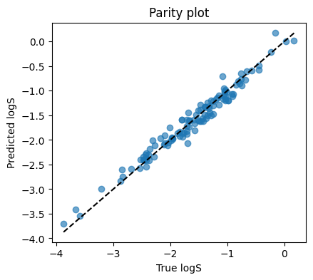
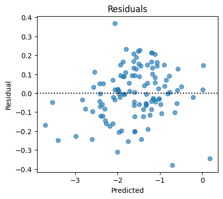
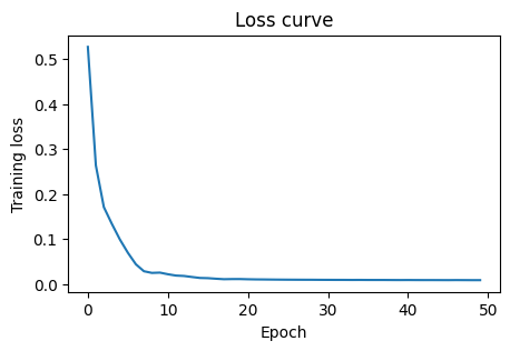
3.3 Parity and training curve

MLPRegressor exposes loss_curve_ after fit. This is the average loss per epoch on the training data.

Compare with lasso (optimized with alpha = 0.1) we learned in Lecture 5, you can see its performance is better even without optimizing the hyperparameters.

reg1.fit(Xtr, ytr)
yhat = reg1.predict(Xte)

print(f"MSE: {mean_squared_error(yte, yhat):.4f}")
print(f"MAE: {mean_absolute_error(yte, yhat):.4f}")
print(f"R2:  {r2_score(yte, yhat):.3f}")

MSE: 0.0185
MAE: 0.1075
R2:  0.966

Show code cell source

Hide code cell source

plt.figure(figsize=(4.6,4))
plt.scatter(yte, yhat, alpha=0.65)
lims = [min(yte.min(), yhat.min()), max(yte.max(), yhat.max())]
plt.plot(lims, lims, "k--")
plt.xlabel("True logS")
plt.ylabel("Predicted logS")
plt.title("Parity plot")
plt.show()

resid = yte - yhat
plt.figure(figsize=(4.6,4))
plt.scatter(yhat, resid, alpha=0.65)
plt.axhline(0, color="k", linestyle=":")
plt.xlabel("Predicted")
plt.ylabel("Residual")
plt.title("Residuals")
plt.show()

Show code cell source

Hide code cell source

mlp_reg = reg1.named_steps["mlp"]
plt.figure(figsize=(5,3))
plt.plot(mlp_reg.loss_curve_)
plt.xlabel("Epoch")
plt.ylabel("Training loss")
plt.title("Loss curve")
plt.show()

---

4. Classification with MLP on toxicity

Moving beyond regression, let’s look an example on the classification.

We will predict toxic vs non_toxic from the same four descriptors.

4.1 Prepare labels and build classifier

df_clf = df[["MolWt","LogP","TPSA","NumRings","Toxicity"]].dropna()
label_map = {"toxic":1, "non_toxic":0}
y = df_clf["Toxicity"].str.lower().map(label_map).astype(int).values
X = df_clf[["MolWt","LogP","TPSA","NumRings"]].values

Xtr, Xte, ytr, yte = train_test_split(X, y, test_size=0.2, random_state=42, stratify=y)


clf_pipe = Pipeline([
    ("scaler", StandardScaler()),
    ("mlp", MLPClassifier(hidden_layer_sizes=(16,),
                          activation="relu",
                          learning_rate_init=0.01,
                          max_iter=2000,
                          random_state=0))
])
clf_pipe

Pipeline(steps=[('scaler', StandardScaler()),
                ('mlp',
                 MLPClassifier(hidden_layer_sizes=(16,),
                               learning_rate_init=0.01, max_iter=2000,
                               random_state=0))])

In a Jupyter environment, please rerun this cell to show the HTML representation or trust the notebook.
On GitHub, the HTML representation is unable to render, please try loading this page with nbviewer.org.

Everything stays the same except we use MLPClassifier() instead of MLPRegressor()

Now let’s fit and evaluate.

clf_pipe.fit(Xtr, ytr)
yp = clf_pipe.predict(Xte)
yproba = clf_pipe.predict_proba(Xte)[:,1]

acc  = accuracy_score(yte, yp)
prec = precision_score(yte, yp)
rec  = recall_score(yte, yp)
f1   = f1_score(yte, yp)
auc  = roc_auc_score(yte, yproba)

print(f"Accuracy:  {acc:.3f}")
print(f"Precision: {prec:.3f}")
print(f"Recall:    {rec:.3f}")
print(f"F1:        {f1:.3f}")
print(f"AUC:       {auc:.3f}")

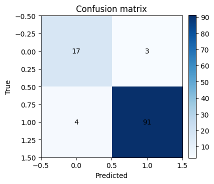
cm = confusion_matrix(yte, yp)
plt.figure(figsize=(4,4))
plt.imshow(cm, cmap="Blues")
plt.title("Confusion matrix")
plt.xlabel("Predicted")
plt.ylabel("True")
for i in range(2):
    for j in range(2):
        plt.text(j, i, cm[i,j], ha="center", va="center")
plt.colorbar(fraction=0.046, pad=0.04)
plt.show()

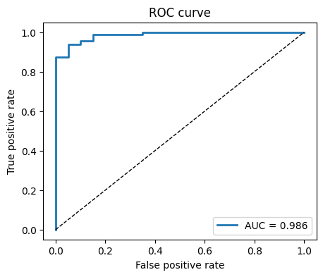
fpr, tpr, thr = roc_curve(yte, yproba)
plt.figure(figsize=(5,4))
plt.plot(fpr, tpr, lw=2, label=f"AUC = {auc:.3f}")
plt.plot([0,1], [0,1], "k--", lw=1)
plt.xlabel("False positive rate")
plt.ylabel("True positive rate")
plt.title("ROC curve")
plt.legend()
plt.show()

Accuracy:  0.939
Precision: 0.968
Recall:    0.958
F1:        0.963
AUC:       0.986

Threshold tuning demo.

for t in [0.3, 0.5, 0.7]:
    yp_t = (yproba >= t).astype(int)
    print(f"threshold={t:.2f}  acc={accuracy_score(yte, yp_t):.3f}  prec={precision_score(yte, yp_t):.3f}  rec={recall_score(yte, yp_t):.3f}")

threshold=0.30  acc=0.965  prec=0.969  rec=0.989
threshold=0.50  acc=0.939  prec=0.968  rec=0.958
threshold=0.70  acc=0.930  prec=0.978  rec=0.937

---

5. Peek inside the network

While scikit-learn MLP is a black box in training, you can still inspect weights.

We will look at the first layer weights for regression on log-solubility and see which descriptors each hidden unit is sensitive to.

reg_inspect = Pipeline([
    ("scaler", StandardScaler()),
    ("mlp", MLPRegressor(hidden_layer_sizes=(8,),
                         activation="tanh",
                         learning_rate_init=0.01,
                         alpha=1e-3,
                         max_iter=1500,
                         random_state=0))
]).fit(Xtr, ytr)

W1 = reg_inspect.named_steps["mlp"].coefs_[0]  # shape (4, 8)
cols = ["MolWt","LogP","TPSA","NumRings"]

plt.figure(figsize=(6,3.5))
plt.imshow(W1, aspect="auto", cmap="bwr")
plt.yticks(range(len(cols)), cols)
plt.xticks(range(W1.shape[1]), [f"h{j}" for j in range(W1.shape[1])])
plt.colorbar(label="weight")
plt.title("First layer weights")
plt.show()

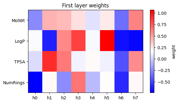
How to read above plot:

Each column is a hidden unit. Positive weights mean the unit activates when that feature is larger than average. Negative weights mean the opposite. This is not a full explanation, but it gives a flavor of what the network latches onto.

⏰ Exercises 5

Try to overwrite the Xtr, ytr with different task (e.g. melting point regression, solubility regression, toxicity classification) and use different MLP to see the difference.

---

6. Overfitting, regularization, and early stopping

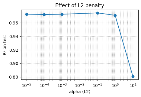
Neural nets can overfit small chemistry tables. Two easy controls:

• L2 penalty via alpha. Larger alpha shrinks weights.

• Early stopping stops when validation score stops improving.

We will show a sweep of alpha for log-solubility.

Show code cell source

Hide code cell source

#reload and overwrite solubility training set
X = df_sol[["MolWt","LogP","TPSA","NumRings"]].values
y = df_sol["logS"].values

Xtr, Xte, ytr, yte = train_test_split(X, y, test_size=0.2, random_state=0)

alphas = [1e-5, 1e-4, 1e-3, 1e-1, 1, 10]
scores = []
for a in alphas:
    reg = Pipeline([
        ("scaler", StandardScaler()),
        ("mlp", MLPRegressor(hidden_layer_sizes=(32,),
                             activation="relu",
                             learning_rate_init=0.01,
                             alpha=a,
                             early_stopping=True,
                             validation_fraction=0.15,
                             max_iter=3000,
                             random_state=0))
    ])
    reg.fit(Xtr, ytr)
    yhat = reg.predict(Xte)
    scores.append(r2_score(yte, yhat))

pd.DataFrame({"alpha": alphas, "R2": np.round(scores, 4)})

plt.figure(figsize=(5,3))
plt.semilogx(alphas, scores, marker="o")
plt.xlabel("alpha (L2)")
plt.ylabel("R² on test")
plt.title("Effect of L2 penalty")
plt.grid(True, which="both", linestyle=":")
plt.show()

---

7. Glossary

multilayer perceptron

A network of layers that apply linear transforms plus nonlinear activations.

activation

Nonlinear function applied elementwise. Common choices: ReLU, tanh, logistic.

loss

A number that measures how wrong the predictions are on training data.

optimizer

Method that updates weights to reduce loss. Scikit-learn uses variants of SGD or LBFGS under the hood.

alpha

L2 penalty strength in scikit-learn MLP. Larger means more shrinkage.

early stopping

Stop training when validation score does not improve for a patience window.

scaling

Standardize features to zero mean and unit variance. Critical for neural nets.

parity plot

Scatter of predicted vs true values for regression.

ROC AUC

Area under the Receiver Operating Characteristic curve. Threshold free ranking metric.

hidden layer

A layer between input and output that lets the model learn nonlinear combinations.

---

8. Quick reference

Recipes

• Always scale inputs for MLPs: Pipeline([("scaler", StandardScaler()), ("mlp", ...)])

• Start small: one hidden layer with 16 to 64 units

• For regression: check parity and residual plots

• For classification: look at confusion matrix and ROC

• To avoid overfitting: increase alpha and use early_stopping=True

• Reproducibility: set random_state

Common args

• hidden_layer_sizes=(h1, h2, ...) number of units per layer

• activation="relu" or "tanh"

• alpha L2 penalty, try 1e-5 to 1e-2

• learning_rate_init step size, try 0.001 to 0.05

• max_iter cap on epochs

• early_stopping=True and validation_fraction=0.1 to 0.2

---

9. In-class activity

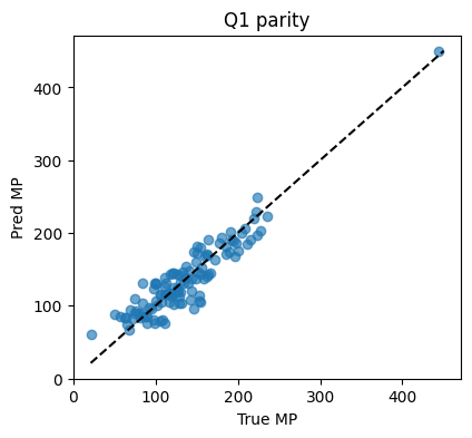
Q1. Tiny MLP for melting point

• Use features [MolWt, LogP, TPSA, NumRings]

• Split 80/20 with random_state=7

• Train MLPRegressor with (32,), alpha=1e-3, ReLU

• Report MSE, MAE, R² and draw a parity plot

# Q1 starter
...


df_reg = df[["MolWt","LogP","TPSA","NumRings","Melting Point"]].dropna()
X = df_reg[["MolWt","LogP","TPSA","NumRings"]].values
y = df_reg["Melting Point"].values

Xtr, Xte, ytr, yte = train_test_split(...) #TO DO

pipe = Pipeline(...).fit(Xtr, ytr)  #TO DO

yhat = pipe.predict(Xte)
print(f"MSE={mean_squared_error(yte,yhat):.2f}  MAE={mean_absolute_error(yte,yhat):.2f}  R2={r2_score(yte,yhat):.3f}")

plt.figure(figsize=(4.5,4))
plt.scatter(yte, yhat, alpha=0.65)
lims = [min(yte.min(), yhat.min()), max(yte.max(), yhat.max())]
plt.plot(lims, lims, "k--")
plt.xlabel("True MP"); plt.ylabel("Pred MP"); plt.title("Q1 parity")
plt.show()

---

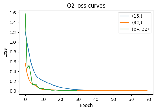
Q2. Depth vs width on log-solubility

• Train three models on logS with hidden sizes (16,), (32,), (64,32)

• Keep alpha=1e-3, learning_rate_init=0.01, early stopping on

• Compare test R² and plot the three loss curves on the same plot

# Q2 starter

df_sol = df[["MolWt","LogP","TPSA","NumRings","Solubility_mol_per_L"]].dropna().copy()
df_sol["logS"] = np.log10(df_sol["Solubility_mol_per_L"]+1e-6)
X = df_sol[["MolWt","LogP","TPSA","NumRings"]].values
y = df_sol["logS"].values

Xtr, Xte, ytr, yte = train_test_split(X, y, test_size=0.2, random_state=15)

sizes = [...] #TO DO
r2s, curves = [], []


for sz in sizes:
    pipe = Pipeline([
        ("scaler", StandardScaler()),
        ("mlp", MLPRegressor(hidden_layer_sizes=sz, activation="relu",
                             alpha=...,  #TO DO
                             learning_rate_init=...,  #TO DO
                             early_stopping=..., #TO DO
                             validation_fraction=0.15,
                             max_iter=3000, random_state=0))
    ]).fit(Xtr, ytr)
    yhat = pipe.predict(Xte)
    r2s.append(r2_score(yte, yhat))
    curves.append(pipe.named_steps["mlp"].loss_curve_)

print(pd.DataFrame({"hidden_sizes":[str(s) for s in sizes],"R2":np.round(r2s,3)}))

plt.figure(figsize=(5.5,3.5))
for sz, c in zip(sizes, curves):
    plt.plot(c, label=str(sz))
plt.xlabel("Epoch"); plt.ylabel("Loss"); plt.title("Q2 loss curves")
plt.legend(); plt.show()

---

Q3. Toxicity classification with threshold tuning

• For Toxicity, train MLPClassifier with (32,), alpha=1e-3, early stopping on

• Compute probabilities on test

• For thresholds [0.3, 0.5, 0.7] print Accuracy, Precision, Recall, F1

#TO DO

---

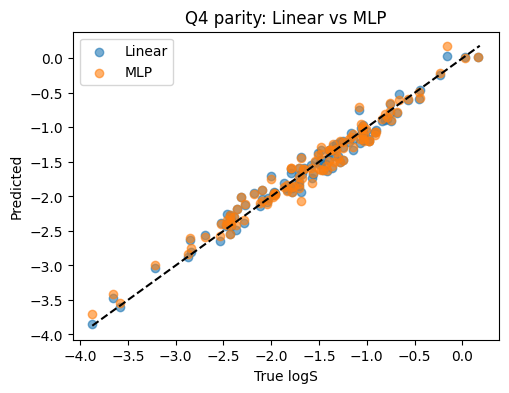
Q4. Compare MLP to Linear Regression on logS

• Same train test split as Q2

• Fit Linear Regression on scaled inputs for logS

• Report both R² on test and draw both parity scatters on one plot

# TO DO

11. Solutions

Solution Q1

df_reg = df[["MolWt","LogP","TPSA","NumRings","Melting Point"]].dropna()
X = df_reg[["MolWt","LogP","TPSA","NumRings"]].values
y = df_reg["Melting Point"].values
Xtr, Xte, ytr, yte = train_test_split(X, y, test_size=0.2, random_state=7)

pipe = Pipeline([
    ("scaler", StandardScaler()),
    ("mlp", MLPRegressor(hidden_layer_sizes=(32,), activation="relu",
                         alpha=1e-3, learning_rate_init=0.01,
                         max_iter=1500, random_state=0))
]).fit(Xtr, ytr)

yhat = pipe.predict(Xte)
print(f"MSE={mean_squared_error(yte,yhat):.2f}  MAE={mean_absolute_error(yte,yhat):.2f}  R2={r2_score(yte,yhat):.3f}")

plt.figure(figsize=(4.5,4))
plt.scatter(yte, yhat, alpha=0.65)
lims = [min(yte.min(), yhat.min()), max(yte.max(), yhat.max())]
plt.plot(lims, lims, "k--")
plt.xlabel("True MP"); plt.ylabel("Pred MP"); plt.title("Q1 parity")
plt.show()

MSE=409.35  MAE=16.27  R2=0.855

Solution Q2

sizes = [(16,), (32,), (64,32)]
df_sol = df[["MolWt","LogP","TPSA","NumRings","Solubility_mol_per_L"]].dropna().copy()
df_sol["logS"] = np.log10(df_sol["Solubility_mol_per_L"]+1e-6)
X = df_sol[["MolWt","LogP","TPSA","NumRings"]].values
y = df_sol["logS"].values
Xtr, Xte, ytr, yte = train_test_split(X, y, test_size=0.2, random_state=15)

r2s, curves = [], []
for sz in sizes:
    reg = Pipeline([
        ("scaler", StandardScaler()),
        ("mlp", MLPRegressor(hidden_layer_sizes=sz, activation="relu",
                             alpha=1e-3, learning_rate_init=0.01,
                             early_stopping=True, validation_fraction=0.15,
                             max_iter=3000, random_state=0))
    ]).fit(Xtr, ytr)
    yhat = reg.predict(Xte)
    r2s.append(r2_score(yte, yhat))
    curves.append(reg.named_steps["mlp"].loss_curve_)

print(pd.DataFrame({"hidden_sizes":[str(s) for s in sizes],"R2":np.round(r2s,3)}))

plt.figure(figsize=(5.5,3.5))
for sz, c in zip(sizes, curves):
    plt.plot(c, label=str(sz))
plt.xlabel("Epoch"); plt.ylabel("Loss"); plt.title("Q2 loss curves")
plt.legend(); plt.show()

  hidden_sizes     R2
0        (16,)  0.950
1        (32,)  0.964
2     (64, 32)  0.958

Solution Q3

df_clf = df[["MolWt","LogP","TPSA","NumRings","Toxicity"]].dropna()
y = df_clf["Toxicity"].str.lower().map({"toxic":1,"non_toxic":0}).astype(int).values
X = df_clf[["MolWt","LogP","TPSA","NumRings"]].values
Xtr, Xte, ytr, yte = train_test_split(X, y, test_size=0.2, random_state=42, stratify=y)

clf = Pipeline([
    ("scaler", StandardScaler()),
    ("mlp", MLPClassifier(hidden_layer_sizes=(32,), activation="relu",
                          alpha=1e-3, learning_rate_init=0.01,
                          early_stopping=True, validation_fraction=0.15,
                          max_iter=3000, random_state=0))
]).fit(Xtr, ytr)

proba = clf.predict_proba(Xte)[:,1]
for t in [0.3, 0.5, 0.7]:
    pred = (proba >= t).astype(int)
    print(f"t={t:.1f}  acc={accuracy_score(yte,pred):.3f}  prec={precision_score(yte,pred):.3f}  rec={recall_score(yte,pred):.3f}  f1={f1_score(yte,pred):.3f}")

t=0.3  acc=0.887  prec=0.887  rec=0.989  f1=0.935
t=0.5  acc=0.896  prec=0.946  rec=0.926  f1=0.936
t=0.7  acc=0.878  prec=0.976  rec=0.874  f1=0.922

Solution Q4

df_sol = df[["MolWt","LogP","TPSA","NumRings","Solubility_mol_per_L"]].dropna().copy()
df_sol["logS"] = np.log10(df_sol["Solubility_mol_per_L"]+1e-6)
X = df_sol[["MolWt","LogP","TPSA","NumRings"]].values
y = df_sol["logS"].values
Xtr, Xte, ytr, yte = train_test_split(X, y, test_size=0.2, random_state=15)

sc = StandardScaler().fit(Xtr)
Xtr_s, Xte_s = sc.transform(Xtr), sc.transform(Xte)

lr = LinearRegression().fit(Xtr_s, ytr)
yhat_lr = lr.predict(Xte_s)

mlp = MLPRegressor(hidden_layer_sizes=(32,), activation="relu",
                   alpha=1e-3, learning_rate_init=0.01,
                   max_iter=3000, random_state=0).fit(Xtr_s, ytr)
yhat_mlp = mlp.predict(Xte_s)

print(f"Linear R2: {r2_score(yte, yhat_lr):.3f}")
print(f"MLP    R2: {r2_score(yte, yhat_mlp):.3f}")

plt.figure(figsize=(5.5,4))
plt.scatter(yte, yhat_lr, alpha=0.6, label="Linear")
plt.scatter(yte, yhat_mlp, alpha=0.6, label="MLP")
lims = [min(yte.min(), yhat_lr.min(), yhat_mlp.min()), max(yte.max(), yhat_lr.max(), yhat_mlp.max())]
plt.plot(lims, lims, "k--")
plt.xlabel("True logS"); plt.ylabel("Predicted")
plt.legend(); plt.title("Q4 parity: Linear vs MLP")
plt.show()

Linear R2: 0.970
MLP    R2: 0.966

Solution Q5

# Solution Q5 (full run + metrics + plots)

import torch, torch.nn as nn
from torch.utils.data import Dataset, DataLoader

# Data
df_mp = df[["MolWt","LogP","TPSA","NumRings","Melting Point"]].dropna().copy()

X = df_mp[["MolWt","LogP","TPSA","NumRings"]].values.astype(np.float32)
y = df_mp["Melting Point"].values.astype(np.float32).reshape(-1,1)

Xtr, Xte, ytr, yte = train_test_split(X, y, test_size=0.2, random_state=15)
scaler = StandardScaler().fit(Xtr)
Xtr_s = scaler.transform(Xtr).astype(np.float32)
Xte_s = scaler.transform(Xte).astype(np.float32)

class NumpyDataset(Dataset):
    def __init__(self, X, y):
        self.X = torch.from_numpy(X)
        self.y = torch.from_numpy(y)
    def __len__(self): return len(self.X)
    def __getitem__(self, i): return self.X[i], self.y[i]

train_loader = DataLoader(NumpyDataset(Xtr_s, ytr), batch_size=64, shuffle=True)

in_dim = Xtr_s.shape[1]
model = nn.Sequential(
    nn.Linear(in_dim, 32), nn.ReLU(),
    nn.Linear(32, 16),     nn.ReLU(),
    nn.Linear(16, 1)
)

loss_fn = nn.MSELoss()
opt = torch.optim.Adam(model.parameters(), lr=1e-3, weight_decay=1e-3)

train_losses = []
model.train()
for epoch in range(200):
    batch_losses = []
    for xb, yb in train_loader:
        pred = model(xb)
        loss = loss_fn(pred, yb)
        opt.zero_grad(); loss.backward(); opt.step()
        batch_losses.append(loss.item())
    train_losses.append(np.mean(batch_losses))

# Evaluate
model.eval()
with torch.no_grad():
    yhat = model(torch.from_numpy(Xte_s)).numpy()

print(f"MSE: {mean_squared_error(yte, yhat):.3f}")
print(f"MAE: {mean_absolute_error(yte, yhat):.3f}")
print(f"R2:  {r2_score(yte, yhat):.3f}")

# Learning curve
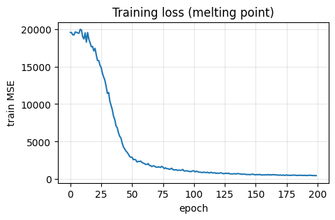
plt.figure(figsize=(5,3))
plt.plot(train_losses)
plt.xlabel("epoch"); plt.ylabel("train MSE"); plt.title("Training loss (melting point)")
plt.grid(alpha=0.3)
plt.show()

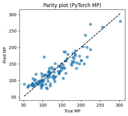
# Parity plot
plt.figure(figsize=(4.6,4))
plt.scatter(yte, yhat, alpha=0.65)
lims = [min(yte.min(), yhat.min()), max(yte.max(), yhat.max())]
plt.plot(lims, lims, "k--")
plt.xlabel("True MP"); plt.ylabel("Pred MP"); plt.title("Parity plot (PyTorch MP)")
plt.show()

MSE: 490.851
MAE: 17.622
R2:  0.769