Lecture 6 - Cross-Validation

Lecture 6 - Cross-Validation#

Learning goals #

Use KFold and cross_val_score for fair evaluation.
Tune hyperparameters with GridSearchCV.
Explain predictions using feature importance and permutation importance.

We will reuse the same table from Lecture 5. It includes SMILES plus targets such as Melting Point and Toxicity. We compute four lightweight descriptors that we already trust: MolWt, LogP, TPSA, NumRings. They are fast to compute, easy to interpret, and good enough to demonstrate model selection and cross‑validation.

1.1 Imports and environment#

1.2 Load data and build descriptors#

Data source

We will use this C-H oxidation dataset we saw before:
https://raw.githubusercontent.com/zzhenglab/ai4chem/main/book/_data/C_H_oxidation_dataset.csv

url = "https://raw.githubusercontent.com/zzhenglab/ai4chem/main/book/_data/C_H_oxidation_dataset.csv"
df_raw = pd.read_csv(url)

def calc_descriptors_row(smiles):
  m = Chem.MolFromSmiles(smiles)
  if m is None:
    return pd.Series({"MolWt": np.nan, "LogP": np.nan, "TPSA": np.nan, "NumRings": np.nan})
  return pd.Series({
            "MolWt": Descriptors.MolWt(m),
            "LogP": Crippen.MolLogP(m),
            "TPSA": rdMolDescriptors.CalcTPSA(m),
            "NumRings": rdMolDescriptors.CalcNumRings(m),
        })


desc_df = df_raw["SMILES"].apply(calc_descriptors_row)
df_reg_mp = pd.concat([df_raw, desc_df], axis=1)
df_reg_mp.head()

	Compound Name	CAS	SMILES	Solubility_mol_per_L	pKa	Toxicity	Melting Point	Reactivity	Oxidation Site	MolWt	LogP	TPSA	NumRings
0	3,4-dihydro-1H-isochromene	493-05-0	c1ccc2c(c1)CCOC2	0.103906	5.80	non_toxic	65.8	1	8,10	134.178	1.7593	9.23	2.0
1	9H-fluorene	86-73-7	c1ccc2c(c1)Cc1ccccc1-2	0.010460	5.82	toxic	90.0	1	7	166.223	3.2578	0.00	3.0
2	1,2,3,4-tetrahydronaphthalene	119-64-2	c1ccc2c(c1)CCCC2	0.020589	5.74	toxic	69.4	1	7,10	132.206	2.5654	0.00	2.0
3	ethylbenzene	100-41-4	CCc1ccccc1	0.048107	5.87	non_toxic	65.0	1	1,2	106.168	2.2490	0.00	1.0
4	cyclohexene	110-83-8	C1=CCCCC1	0.060688	5.66	non_toxic	96.4	1	3,6	82.146	2.1166	0.00	1.0

What these features mean

MolWt: molecular weight (sum of atomic masses).
LogP: hydrophobicity descriptor (octanol/water partition).
TPSA: topological polar surface area.
NumRings: ring count.

2. Quick Exploratory Data Analysis (EDA)#

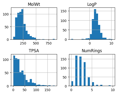
2.1 Descriptor histograms#

Goal

Check scale, spread, and any extreme values. If a feature is highly skewed, consider transforms or standardization before training.

features = ["MolWt", "LogP", "TPSA", "NumRings"]
ax = df_reg_mp[features].hist(bins=20, figsize=(5,4))
plt.tight_layout()
plt.show()

_images/182d8368dce923628285fec322bdccc65c100640960f10ab6270a37ccae0f9b4.png

2.2 Pairwise relationships#

pd.plotting.scatter_matrix(df_reg_mp[features], figsize=(5,5))
plt.suptitle("Descriptor scatter matrix", y=1.02)
plt.show()

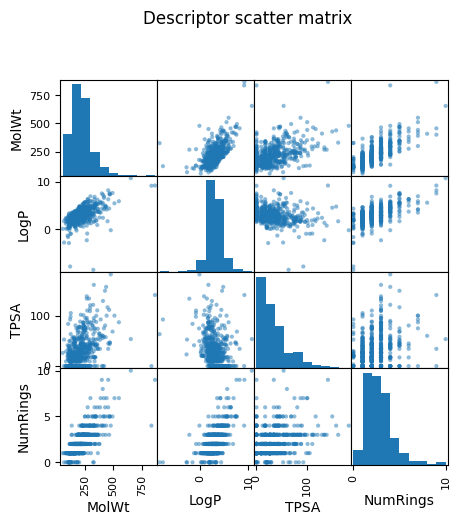
_images/365c7e04c443660fc8973b08118f2eddf704524f1f8e6bb443eac39ff43257a7.png

As you see above, a pairwise plot (also called a scatterplot matrix) shows relationships between every possible pair of features. For example, if you have four descriptors — MolWt, LogP, TPSA, and NumRings — the matrix will draw 12 scatterplots pairs (diagonal being their own distribution).

Why we look at pairwise plots?

Spot correlations: If two descriptors are strongly correlated (for example, heavier molecules often have higher logP), you can see it visually. Highly correlated pairs may be redundant.

Detect outliers: Points that are far away from the general cloud of data stand out.

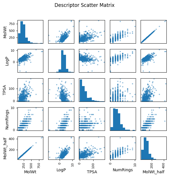
2.3 Redundancy demo and correlation#

To illustrate what redundancy looks like, in the following example, we added a synthetic feature called MolWt_half, created simply by multiplying molecular weight by 0.5. In the scatter matrix, MolWt_half and MolW form a perfect straight-line relationship, highlighting redundancy.

In real-world datasets, you might encounter similar situations where two measured properties track one another closely because they arise from the same underlying physical or chemical trend. In such cases, redundancy reduces the effective dimensionality of the dataset.

This visual impression can be confirmed by calculating the correlation coefficient numerically. A correlation near 1.0 (or –1.0) indicates strong redundancy, just like we see between MolWt and MolWt_half.

# Add demo redundant feature
df_reg_mp["MolWt_half"] = df_reg_mp["MolWt"] * 0.5

# Choose features to visualize
features = ["MolWt", "LogP", "TPSA", "NumRings", "MolWt_half"]

# Numerical correlation matrix
print("\nCorrelation Matrix (rounded to 3 decimals):")
corr_matrix = df_reg_mp[features].corr().round(3)
print(corr_matrix)

# Scatter matrix
pd.plotting.scatter_matrix(df_reg_mp[features], figsize=(6,6), diagonal="hist")
plt.suptitle("Descriptor Scatter Matrix", y=1.02)
plt.tight_layout()
plt.show()

Correlation Matrix (rounded to 3 decimals):
            MolWt   LogP   TPSA  NumRings  MolWt_half
MolWt       1.000  0.595  0.447     0.759       1.000
LogP        0.595  1.000 -0.268     0.605       0.595
TPSA        0.447 -0.268  1.000     0.294       0.447
NumRings    0.759  0.605  0.294     1.000       0.759
MolWt_half  1.000  0.595  0.447     0.759       1.000

_images/a87c79b6ca2b03d61872518e69d4b55dc937a05e55234efa23856261b2901b51.png

3. Introduction to hyperparameters #

Lasso refresher

Lasso solves a linear regression with an L1 penalty. The loss (on a dataset of size n) is
[ \frac{1}{n}\sum_{i=1}^n (y_i - \hat{y}_i)^2 + \alpha \sum_j |w_j| ]
When (\alpha) is larger, more coefficients go to zero.

3.1 Single split evaluation#

When we fit a model, we often think about weights (w) that are learned from the data. But some knobs are not learned automatically — they are chosen by us. These are called hyperparameters. One of the most important hyperparameters in Lasso is alpha. As you may recall from last lecture, it controls the strength of the L1 penalty.

# Define X (features) and y (target)
X = df_reg_mp[["MolWt", "LogP", "TPSA", "NumRings"]]
y = df_reg_mp["Melting Point"]

# Split into train (80%) and test (20%) sets
X_train, X_test, y_train, y_test = train_test_split(
    X, y, test_size=0.2, random_state=1
)

# Define models in a dictionary
models = {
    "Linear Regression": LinearRegression(),
    "Lasso (alpha=0.1)": Lasso(alpha=0.1, max_iter=500),
    "Lasso (alpha=1)":   Lasso(alpha=1,   max_iter=500),
    "Lasso (alpha=10)":  Lasso(alpha=10,  max_iter=500),
    "Lasso (alpha=100)": Lasso(alpha=100, max_iter=500),
    "Lasso (alpha=500)": Lasso(alpha=500, max_iter=500)
}

# Collect results
results = []

for name, model in models.items():
    model.fit(X_train, y_train)
    y_pred = model.predict(X_test)

    mse_val = mean_squared_error(y_test, y_pred)
    mae_val = mean_absolute_error(y_test, y_pred)
    r2_val  = r2_score(y_test, y_pred)

    results.append([name, mse_val, mae_val, r2_val])

# Put results in a nice DataFrame
df_results = pd.DataFrame(results, columns=["Model", "MSE", "MAE", "R2"])
df_results

	Model	MSE	MAE	R2
0	Linear Regression	398.206541	16.006228	0.816101
1	Lasso (alpha=0.1)	396.546775	15.975604	0.816868
2	Lasso (alpha=1)	389.603474	15.816549	0.820074
3	Lasso (alpha=10)	390.347484	15.855184	0.819731
4	Lasso (alpha=100)	399.273984	16.080242	0.815608
5	Lasso (alpha=500)	423.683879	16.757040	0.804335

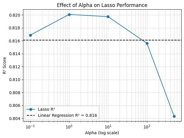
3.2 Effect of alpha (plot)#

# Extract results for plotting
lasso_results = df_results[df_results["Model"].str.contains("Lasso")]
alphas = [0.1, 1, 10, 100, 500]
r2_scores = lasso_results["R2"].values

# Linear Regression baseline
linear_r2 = df_results.loc[df_results["Model"] == "Linear Regression", "R2"].values[0]

# Plot R² vs alpha
plt.figure(figsize=(7,5))
plt.semilogx(alphas, r2_scores, marker="o", label="Lasso R²")
plt.axhline(linear_r2, color="k", linestyle="--", label=f"Linear Regression R² = {linear_r2:.3f}")

plt.xlabel("Alpha (log scale)")
plt.ylabel("R² Score")
plt.title("Effect of Alpha on Lasso Performance")
plt.legend()
plt.grid(True, which="both", linestyle="--", alpha=0.6)
plt.show()

_images/5a196ebf7c869c4daf753f2c1d7b230e6190d744d609503c363d0c7b766ca35c.png

4. Cross validation #

So far we evaluated models with a single 80/20 split, which can give performance estimates that depend strongly on the random split. To obtain a more reliable measure, we can use 4-fold cross validation*. This way, the dataset is split into 4 equal parts, and each part is used once as the test set while the other 3 parts are used for training. The metrics are then averaged across the 4 folds.

Why CV?

A single split can overestimate or underestimate performance. K-fold CV repeats the split several times and averages the metric, giving a more stable estimate.

alphas = [0.1, 1, 10, 100]
kf = KFold(n_splits=4, shuffle=True, random_state=1)

for a in alphas:
    model = Lasso(alpha=a, max_iter=500)
    scores = cross_val_score(model, X, y, cv=kf, scoring="r2")
    print(f"alpha={a}, Scores on each fold: {scores} \n mean R²={scores.mean():.5f} \n")

alpha=0.1, Scores on each fold: [0.80086458 0.8800675  0.85024608 0.81400961] 
 mean R²=0.83630 

alpha=1, Scores on each fold: [0.8012391  0.88025613 0.85027326 0.81361778] 
 mean R²=0.83635 

alpha=10, Scores on each fold: [0.80123962 0.88012751 0.85111665 0.81276335] 
 mean R²=0.83631 

alpha=100, Scores on each fold: [0.79943866 0.87767314 0.85590684 0.80952064] 
 mean R²=0.83563 

Exercise 4.1

Change the alphas to [0.05, 0.5, 1, 2, 5, 15, 30, 100].
Use 5-fold CV and the neg_mean_squared_error scorer.
Print the per-fold values and the mean MSE.

5. Model selection, evaluation and prediction #

Plan

Pick an alpha using CV, fit on train, evaluate on held‑out test, then apply to new molecules.

from sklearn.model_selection import KFold, cross_validate

# Define X and y again
X = df_reg_mp[["MolWt", "LogP", "TPSA", "NumRings"]]
y = df_reg_mp["Melting Point"]

# Train/test split
X_train, X_test, y_train, y_test = train_test_split(X, y, test_size=0.2, random_state=1)

# Use 4-fold cross validation
kf = KFold(n_splits=4, shuffle=True, random_state=1)

# Same models as before
models = {
    "Linear Regression": LinearRegression(),
    "Lasso (alpha=0.1)": Lasso(alpha=0.1, max_iter=500),
    "Lasso (alpha=1)":   Lasso(alpha=1,   max_iter=500),
    "Lasso (alpha=10)":  Lasso(alpha=10,  max_iter=500),
    "Lasso (alpha=30)": Lasso(alpha=30, max_iter=500),
    "Lasso (alpha=100)": Lasso(alpha=100, max_iter=500)
}

results_cv = []

for name, model in models.items():
    cv_results = cross_validate(
        model, X_train, y_train,
        cv=kf,
        scoring=["r2", "neg_mean_squared_error", "neg_mean_absolute_error"],
        return_train_score=False
    )

    # Compute mean and std across folds
    mean_r2 = cv_results["test_r2"].mean()
    mean_mse = -cv_results["test_neg_mean_squared_error"].mean()
    mean_mae = -cv_results["test_neg_mean_absolute_error"].mean()

    results_cv.append([name, mean_mse, mean_mae, mean_r2])

# Put results in a DataFrame
df_results_cv = pd.DataFrame(results_cv, columns=["Model", "MSE", "MAE", "R2"])
print(df_results_cv)

               Model         MSE        MAE        R2
Linear Regression  410.132745  15.969645  0.832197
Lasso (alpha=0.1)  409.638038  15.958751  0.832326
  Lasso (alpha=1)  408.902710  15.918428  0.832658
 Lasso (alpha=10)  408.189050  15.900646  0.833132
 Lasso (alpha=30)  408.099029  15.906188  0.833208
Lasso (alpha=100)  408.969334  15.961744  0.832932

Based on above table, you know alpha = 30 works best for this case. Let’s assign this value to build a model, fit with data and evaluate the outcome, which can be completed within three lines.

alpha_optimized_model = Lasso(alpha=30, max_iter=500)
fitted_lasso = alpha_optimized_model.fit(X_train, y_train)

print(f"Test R² = {r2_score(y_test, fitted_lasso.predict(X_test)):.3f} when we use alpha = 30")

Test R² = 0.818 when we use alpha = 30

R² = 0.820 tells us how good the fitting is. Note this R² is calculated based on the final hold-out test set, so it will be different from the R² one we see during the CV (0.833). The fact that they are very similar to each other is a good sign because this model has never seen any datapoint from X_test before but can still do a good prediction.

Now we can use this function to give prediction for points that are neither in train and test data set. For example, we can predict two molecules’s melting point by listing their descriptors.

Predict new points

We can predict from raw descriptors, or compute descriptors from SMILES first (see example below).

fitted_lasso.predict(pd.DataFrame([[100, 1.5, 10, 2],
                                   [150, 2.0, 20, 3]],
                                  columns=["MolWt", "LogP", "TPSA", "NumRings"]))

array([70.44917852, 95.30123863])

smiles_list = ["C1CCCC(C)C1", "CCCO"]

# Explicitly call your function for each SMILES
desc_rows = [calc_descriptors_row(s) for s in smiles_list]

# Build DataFrame
new_desc = pd.DataFrame(desc_rows)
new_desc

	MolWt	LogP	TPSA	NumRings
0	98.189	2.5866	0.00	1.0
1	60.096	0.3887	20.23	0.0

# Predict
two_new_preds = fitted_lasso.predict(new_desc)

# Show results
results = pd.DataFrame({"SMILES": smiles_list, "Prediction": two_new_preds})
print(results)

        SMILES  Prediction
0  C1CCCC(C)C1   69.345037
1         CCCO   51.000708

If your combine all above together, the workflow will look like:

Define features and target (MolWt, LogP, TPSA, NumRings → Melting Point).
Split data: 80% train, 20% test.
Model selection

Last lecture: fit on train directly if no hyperparameter tuning needed.
Lasso Regression (this lecture): use 4-fold cross-validation on train to pick best alpha, then refit on full train.

Evaluate chosen model on test set for generalization.
Apply final model to new molecules for prediction.

6. End‑to‑end workflow and grid search #

Two ways to choose alpha

Manual loop over a grid and pick the best mean CV score.
GridSearchCV to automate the loop, scoring, and refit.

# 1) Features and target
X = df_reg_mp[["MolWt", "LogP", "TPSA", "NumRings"]]
y = df_reg_mp["Melting Point"]

# 2) Train/test split
X_train, X_test, y_train, y_test = train_test_split(X, y, test_size=0.2, random_state=1)

# 3 Choose alpha using 4-fold CV on TRAIN ONLY
alphas = [0.05, 0.1, 0.3, 0.5, 0.75, 1, 1.5, 2, 3, 5, 10,
          15, 20, 25, 30, 35, 40, 45, 50, 75, 100, 150, 200]
kf = KFold(n_splits=4, shuffle=True, random_state=1)
mean_r2 = []
for a in alphas:
    model = Lasso(alpha=a, max_iter=500)
    r2_vals = cross_val_score(model, X_train, y_train, cv=kf, scoring="r2")
    mean_r2.append(r2_vals.mean())
best_alpha = alphas[int(np.argmax(mean_r2))]
print(f"Best alpha: {best_alpha} (mean R² = {max(mean_r2):.3f})")

# 4) Fit with best alpha on TRAIN, evaluate on TEST
final_lasso = Lasso(alpha=best_alpha, max_iter=500).fit(X_train, y_train)

# 5) Evaluate
y_pred = final_lasso.predict(X_test)
print(f"Test R² = {r2_score(y_test, y_pred):.3f}")

# Optional: compare to plain Linear Regression
lr = LinearRegression().fit(X_train, y_train)
print(f"Linear Regression Test R² = {r2_score(y_test, lr.predict(X_test)):.3f}")

# Quick plot of the selection
plt.semilogx(alphas, mean_r2, marker="o")
plt.axvline(best_alpha, linestyle=":")
plt.xlabel("Alpha (log)"); plt.ylabel("Mean R² (4-fold on train)"); plt.title("Pick alpha by CV")
plt.show()

Best alpha: 30 (mean R² = 0.833)
Test R² = 0.818
Linear Regression Test R² = 0.816

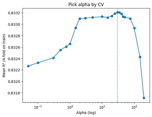
_images/f661b83b89f790f3afe8a0e3fffc1258d7454e3ae5692b31e0697714c20b1a91.png

The block above actually shows a manual grid search: you loop through candidate alphas, run cross-validation, collect mean R² scores, and then pick the best alpha before refitting on the training set.

Now, the second block below shows the same idea implemented with GridSearchCV: it automates the loop, scoring, and best-alpha selection. With refit=True, the best model is automatically retrained on the full training data, so you can directly use grid.best_estimator_ for evaluation.

# 1) Data
X = df_reg_mp[["MolWt", "LogP", "TPSA", "NumRings"]]
y = df_reg_mp["Melting Point"]

# 2) Train/test split
X_train, X_test, y_train, y_test = train_test_split(X, y, test_size=0.2, random_state=1)

# 3a) Define model and CV
lasso = Lasso(max_iter=500)
param_grid = {"alpha": [0.05, 0.1, 0.3, 0.5, 0.75, 1, 1.5, 2, 3, 5,
                        10, 15, 20, 25, 30, 35, 40, 45, 50, 75,
                        100, 150, 200]}
cv = KFold(n_splits=4, shuffle=True, random_state=1)

# 3b) Grid search on TRAIN
grid = GridSearchCV(lasso, param_grid, cv=cv, scoring="r2", refit=True)
grid.fit(X_train, y_train)
print(f"Best alpha: {grid.best_params_['alpha']} (mean R^2 = {grid.best_score_:.3f})")

# 4) Best model (already fitted)
final_lasso = grid.best_estimator_

# 5) Evaluate on TEST
y_pred = final_lasso.predict(X_test)
print(f"Test R^2 = {r2_score(y_test, y_pred):.3f}")

Best alpha: 30 (mean R^2 = 0.833)
Test R^2 = 0.818

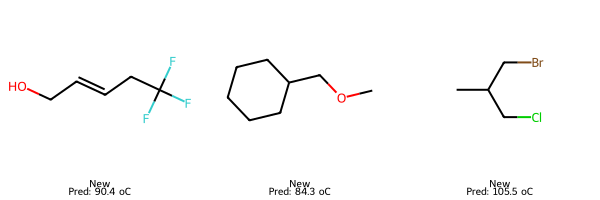
# 5) Predict on new molecules
smiles_three_new = ["C(F)(F)(F)CC=CCO", "C1CCCC(COC)C1", "CC(CBr)CCl"]

# Compute descriptors for each SMILES
smiles_three_new_desc = pd.DataFrame([calc_descriptors_row(s) for s in smiles_three_new])

# Predict for valid rows
smiles_three_new_preds = final_lasso.predict(smiles_three_new_desc)

# Show results
results = pd.DataFrame({"SMILES": np.array(smiles_three_new), "Prediction": smiles_three_new_preds})
print(results.to_string(index=False))

          SMILES  Prediction
C(F)(F)(F)CC=CCO   90.429280
   C1CCCC(COC)C1   84.337454
      CC(CBr)CCl  105.456027

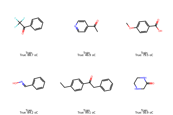
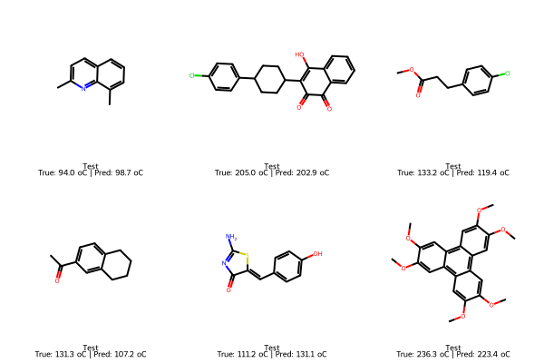
We can also plot some representative molecules in train and test set, as well as some new molecules we want to predict outside the exisiting dataset.

# Pick samples
train_idx = X_train.sample(6, random_state=101).index
test_idx  = X_test.sample(6,  random_state=202).index

# Train: true only
train_smiles = df_reg_mp.loc[train_idx, "SMILES"].tolist()
train_true   = y_train.loc[train_idx].tolist()
img_train = Draw.MolsToGridImage(
    [Chem.MolFromSmiles(s) for s in train_smiles],
    molsPerRow=3, subImgSize=(200,200),
    legends=[f"Train\nTrue: {t:.1f} oC" for t in train_true]
)

# Test: true and predicted
test_smiles = df_reg_mp.loc[test_idx, "SMILES"].tolist()
test_true   = y_test.loc[test_idx].tolist()
test_pred   = final_lasso.predict(X_test.loc[test_idx])
img_test = Draw.MolsToGridImage(
    [Chem.MolFromSmiles(s) for s in test_smiles],
    molsPerRow=3, subImgSize=(200,200),
    legends=[f"Test\nTrue: {t:.1f} oC | Pred: {p:.1f} oC"
             for t,p in zip(test_true, test_pred)]
)

# New: predicted only
smiles_new = ["C(F)(F)(F)CC=CCO", "C1CCCC(COC)C1", "CC(CBr)CCl"]
X_new = pd.DataFrame([calc_descriptors_row(s) for s in smiles_new])[final_lasso.feature_names_in_]
pred_new = final_lasso.predict(X_new)
img_new = Draw.MolsToGridImage(
    [Chem.MolFromSmiles(s) for s in smiles_new],
    molsPerRow=3, subImgSize=(200,200),
    legends=[f"New\nPred: {p:.1f} oC" for p in pred_new]
)

display(img_train); display(img_test); display(img_new)

_images/b42d11431dd71cb1dd14263d0bc3c22f0956d69af1a26ae49c8f09f2f0ccadde.png

_images/b61dc7a5c42de1b5f5a5bfadc3b6232580970109ab9f6e0847fdafe3cd33a389.png

_images/f23605430ae538b2524ffaed859d9e8760516075112406fe19dbe838f0063088.png

7. Explaining the model with feature importance #

Two views

Coefficients: direction and weight (Lasso shrinks some to zero).
Permutation importance: how much test R² drops when a feature is shuffled.

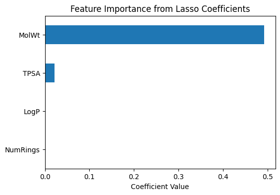
# --- Coefficient-based importance (Lasso) ---
coef_importance = pd.Series(
    final_lasso.coef_,
    index=final_lasso.feature_names_in_
).sort_values(key=abs, ascending=False)

print("Lasso coefficients (feature importance):")
print(coef_importance)

# Plot coefficients
coef_importance.plot(kind="barh", figsize=(6,4))
plt.title("Feature Importance from Lasso Coefficients")
plt.xlabel("Coefficient Value")
plt.gca().invert_yaxis()
plt.show()

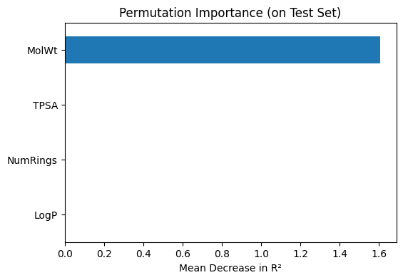
# --- Permutation importance (model agnostic) ---
perm_importance = permutation_importance(
    final_lasso, X_test, y_test,
    scoring="r2", n_repeats=20, random_state=1
)

perm_series = pd.Series(
    perm_importance.importances_mean,
    index=final_lasso.feature_names_in_
).sort_values(ascending=True)

print("\nPermutation importance (mean decrease in R²):")
print(perm_series)

# Plot permutation importance
perm_series.plot(kind="barh", figsize=(6,4))
plt.title("Permutation Importance (on Test Set)")
plt.xlabel("Mean Decrease in R²")
plt.show()

Lasso coefficients (feature importance):
MolWt       0.492808
TPSA        0.021167
LogP       -0.000000
NumRings   -0.000000
dtype: float64

_images/014a98b5151c634dab01b31e406166d7a7636434e440a7ceee670b7c00b82c91.png

Permutation importance (mean decrease in R²):
LogP        0.000000
NumRings    0.000000
TPSA        0.002218
MolWt       1.607811
dtype: float64

_images/4e5b94ff60e08160dab6b4516d8c82c2e9d9018b472b2e6bc4afa1afd88cb437.png

8. Glossary #

Lasso Regression#: Linear regression with L1 regularization that can set some coefficients to exactly zero (feature selection).
Alpha (λ)#: Penalty strength in Lasso. Larger alpha increases regularization and may reduce the number of active features.
Cross validation (CV)#: Split the data into folds, train on k‑1 folds and validate on the held‑out fold; repeat and average.
R² (coefficient of determination)#: Measures how much variance the model explains. 1 is perfect, 0 matches the mean predictor.
MSE#: Mean of squared errors. Sensitive to large errors.
MAE#: Mean of absolute errors. More robust to outliers than MSE.
Permutation importance#: Test‑time feature shuffle to estimate performance drop for each feature.
Coefficient importance#: Weights in a linear model. In Lasso, many are shrunk to 0.
Feature redundancy#: Two or more features carry nearly the same information (high correlation).
GridSearchCV#: Scikit‑learn tool that evaluates parameter grids with CV and returns the best estimator.

9. Quick reference #

Common scikit‑learn patterns

Split: train_test_split(X, y, test_size=0.2, random_state=...)
CV: KFold(n_splits=4, shuffle=True, random_state=...)
Score: cross_val_score(model, X, y, cv=kf, scoring="r2")
Grid search: GridSearchCV(model, {"alpha":[...]}, cv=kf, scoring="r2", refit=True)
Metrics: mean_squared_error, mean_absolute_error, r2_score

Diagnostic plots

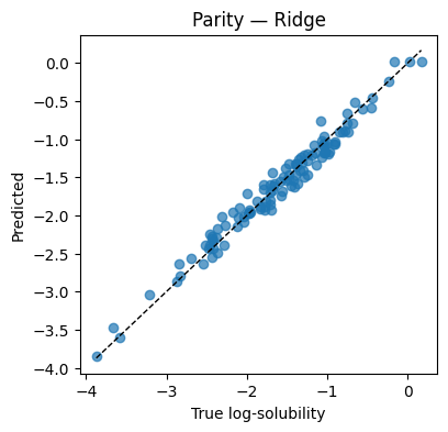
Parity: predicted vs true (should hug the diagonal).
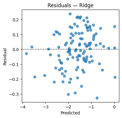
Residuals: residual vs prediction (should center near 0 without pattern).
CV curve: metric vs hyperparameter; pick the stable peak.

10. In‑class activity #

Each task uses the functions and concepts above. Fill in the ... lines.

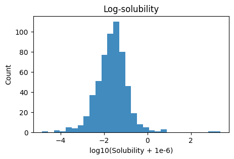
Q1. Prepare log‑solubility and visualize#

Prepare log-solubility, split 80/20 (seed=15), and visualize.

Create y_log· = log10(Solubility_mol_per_L + 1e-6),
Set X = [MolWt, LogP, TPSA, NumRings],
Split 80/20 with random_state=15,
Plot a histogram of y_log, then a pairwise scatter matrix of the four descriptors.

Hint: After spliting, keep t

# TO DO
# y_log = ...
# X = ...
# X_train, X_test, y_train, y_test = train_test_split(X, y_log, test_size=0.2, random_state=15)

# Plots
# ...

Q2. Tune Ridge on the training split#

Search alphas on np.logspace(-2, 3, 12) using 5‑fold CV on (X_tr, y_tr)
Report best alpha and mean CV R², then refit Ridge(alpha=best) on train

# TO DO
# cv = KFold(n_splits=..., shuffle=..., random_state=...)
# alphas = ...
# ...
# ...
# ridge_best = Ridge(alpha=...).fit(..., ...)
# print(f"best alpha={...:.4f}  CV mean R2={max(...):.3f}")

Q3. Evaluate Ridge on test and draw diagnostics#

Compute MSE, MAE, R² on (X_te, y_te)
Plot a parity plot and a residual plot

# TO DO
# y_hat = ...
# print(f"Test MSE={...:.4f}  MAE={...:.4f}  R2={...:.3f}")
# Parity and residual plots
# ...

Q4. Predict two new molecules (Ridge)#

Use the trained Ridge to predict log‑solubility for:

[135.0, 2.0, 9.2, 2]
[301.0, 0.5, 17.7, 2]

# TO DO
# X_new = np.array([[135.0, 2.0, 9.2, 2],
#                   [301.0, 0.5, 17.7, 2]])
# y_new = ridge_best.predict(X_new)
# print(pd.DataFrame({"MolWt": X_new[:,0], "LogP": X_new[:,1], "TPSA": X_new[:,2], "NumRings": X_new[:,3],
#                     "Predicted log10(solubility)": y_new}))

Q5. Interpret Ridge with coefficients and permutation importance#

Show coefficient magnitudes and signs
Compute permutation importance on the test split and plot

# TO DO
# feat = ["MolWt","LogP","TPSA","NumRings"]
# coef_ser = ...
# coef_ser.plot(kind="barh"); ...

# perm = permutation_importance(...)
# perm_ser = ...
# perm_ser.plot(kind="barh"); ...

11. Solutions #

11.1 Solution Q1#

# Log target
df_reg_mp = df_reg_mp.copy()
y_log = np.log10(df_reg_mp["Solubility_mol_per_L"] + 1e-6)

# Features and split
X = df_reg_mp[["MolWt","LogP","TPSA","NumRings"]].values
X_tr, X_te, y_tr, y_te = train_test_split(X, y_log, test_size=0.2, random_state=15)

# Plots
plt.figure(figsize=(5,3))
plt.hist(y_log, bins=30, alpha=0.85)
plt.xlabel("log10(Solubility + 1e-6)"); plt.ylabel("Count"); plt.title("Log-solubility")
plt.show()

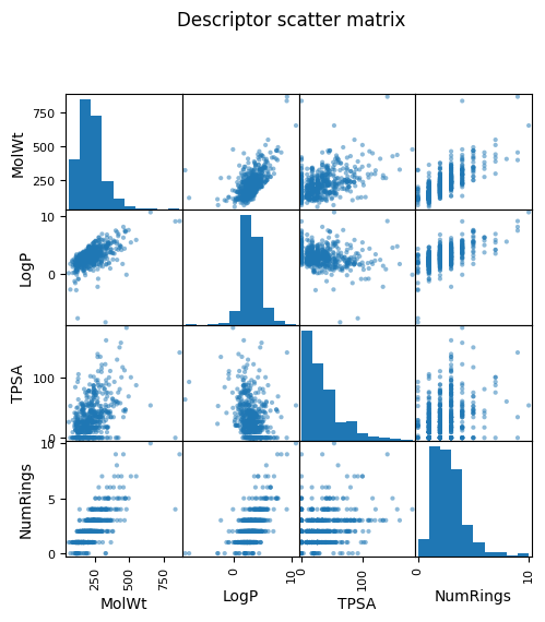
pd.plotting.scatter_matrix(df_reg_mp[["MolWt","LogP","TPSA","NumRings"]], figsize=(5.5,5.5))
plt.suptitle("Descriptor scatter matrix", y=1.02); plt.show()

_images/3ade42a869662442893fa34351be2a4933cd4312213f73a2fd05084ef8a6f692.png

_images/bc9f8070cc3eebdcc189a3046eba2d64baf6368500c4a3de9424b713e51b5598.png

11.2 Solution Q2#

cv = KFold(n_splits=5, shuffle=True, random_state=1)
alphas = np.logspace(-2, 3, 12)
means = [cross_val_score(Ridge(alpha=a), X_tr, y_tr, cv=cv, scoring="r2").mean() for a in alphas]
best_a = float(alphas[int(np.argmax(means))])
ridge_best = Ridge(alpha=best_a).fit(X_tr, y_tr)
print(f"best alpha={best_a:.4f}  CV mean R2={max(means):.3f}")

best alpha=1.8738  CV mean R2=0.968

11.3 Solution Q3#

y_hat = ridge_best.predict(X_te)
print(f"Test MSE={mean_squared_error(y_te,y_hat):.4f}  "
      f"MAE={mean_absolute_error(y_te,y_hat):.4f}  "
      f"R2={r2_score(y_te,y_hat):.3f}")

plt.figure(figsize=(4.2,4))
plt.scatter(y_te, y_hat, alpha=0.7)
lims = [min(y_te.min(), y_hat.min()), max(y_te.max(), y_hat.max())]
plt.plot(lims, lims, "k--", lw=1)
plt.xlabel("True log-solubility"); plt.ylabel("Predicted"); plt.title("Parity — Ridge"); plt.show()

resid = y_te - y_hat
plt.figure(figsize=(4.2,4))
plt.scatter(y_hat, resid, alpha=0.7); plt.axhline(0, color="k", ls=":")
plt.xlabel("Predicted"); plt.ylabel("Residual"); plt.title("Residuals — Ridge"); plt.show()

Test MSE=0.0160  MAE=0.1024  R2=0.970

_images/c17c780964c3bd2393dfe1c3bc464510c8c619a5ffb1c9abee274b7c00876a84.png

_images/09e5082a65c400c82f645abe932b97b9759aa9a460a974f9ea2db1c69274b537.png

11.4 Solution Q4#

X_new = np.array([
    [135.0,  2.0,  9.2, 2],   # Molecule A
    [301.0,  0.5, 17.7, 2]    # Molecule B
])  # descriptors: [MolWt, LogP, TPSA, NumRings]

y_new = ridge_best.predict(X_new)
print(pd.DataFrame({
    "MolWt": X_new[:,0], "LogP": X_new[:,1], "TPSA": X_new[:,2], "NumRings": X_new[:,3],
    "Predicted log10(solubility)": y_new
}))

   MolWt  LogP  TPSA  NumRings  Predicted log10(solubility)
0  135.0   2.0   9.2       2.0                    -1.195502
1  301.0   0.5  17.7       2.0                    -0.501762

11.5 Solution Q5#

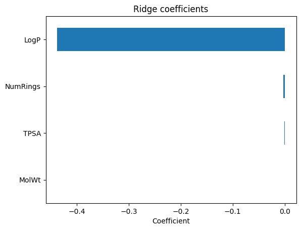
feat = ["MolWt","LogP","TPSA","NumRings"]

coef_ser = pd.Series(ridge_best.coef_, index=feat).sort_values(key=np.abs, ascending=False)
print("Ridge coefficients:\n", coef_ser)
coef_ser.plot(kind="barh"); plt.gca().invert_yaxis()
plt.xlabel("Coefficient"); plt.title("Ridge coefficients"); plt.show()

perm = permutation_importance(ridge_best, X_te, y_te, scoring="r2", n_repeats=30, random_state=1)
perm_ser = pd.Series(perm.importances_mean, index=feat).sort_values()
perm_ser.plot(kind="barh"); plt.xlabel("Mean decrease in R²"); plt.title("Permutation importance on test"); plt.show()

Ridge coefficients:
 LogP       -0.437668
NumRings   -0.002761
TPSA       -0.000699
MolWt       0.000260
dtype: float64

_images/bfaaa5a02eb717b2ec739fff482fa179e7d8398fcf42c479ca837996cdac1def.png

_images/c544f6385c1968c5d3b7e44c1d1ba339e6b863ab85b4abc1676c107926737a95.png