Lecture 7 - Decision Trees and Random Forests

Learning goals

• Explain the intuition of decision trees for regression and classification.

• Read Gini and entropy for splits and MSE for regression splits.

• Grow a tree step by step and inspect internal structures: nodes, depth, leaf counts.

• Control tree growth with max_depth, min_samples_leaf, min_samples_split.

• Visualize a fitted tree and feature importance.

• Train a Random Forest and compare to a single tree.

• Put it all together in a short end-to-end workflow.

  

---

0. Setup

Show code cell source

Hide code cell source

# 0. Setup
import numpy as np
import pandas as pd
import matplotlib.pyplot as plt

try:
    from rdkit import Chem
    from rdkit.Chem import Descriptors, Crippen, rdMolDescriptors
except Exception:
    Chem = None

from sklearn.model_selection import train_test_split
from sklearn.metrics import (
    mean_squared_error, mean_absolute_error, r2_score,
    accuracy_score, precision_score, recall_score, f1_score,
    confusion_matrix, roc_auc_score, roc_curve
)
from sklearn.tree import DecisionTreeRegressor, DecisionTreeClassifier, plot_tree
from sklearn.ensemble import RandomForestRegressor, RandomForestClassifier
from sklearn.inspection import permutation_importance
from sklearn.model_selection import GridSearchCV, KFold, train_test_split
from sklearn.linear_model import LinearRegression, Lasso, Ridge, LogisticRegression, lasso_path
from sklearn.model_selection import train_test_split, KFold, GridSearchCV
from sklearn.metrics import accuracy_score, roc_auc_score, roc_curve
from sklearn.ensemble import RandomForestClassifier

import warnings
warnings.filterwarnings("ignore", message="X does not have valid feature names")
warnings.filterwarnings("ignore", message="X has feature names")

1. Decision tree

1.1 Load data and build descriptors

We will reuse the same dataset to keep the context consistent. If RDKit is available, we compute four descriptors; otherwise we fallback to numeric columns that are already present.

Show code cell source

Hide code cell source

url = "https://raw.githubusercontent.com/zzhenglab/ai4chem/main/book/_data/C_H_oxidation_dataset.csv"
df_raw = pd.read_csv(url)
df_raw.head()

	Compound Name	CAS	SMILES	Solubility_mol_per_L	pKa	Toxicity	Melting Point	Reactivity	Oxidation Site
0	3,4-dihydro-1H-isochromene	493-05-0	c1ccc2c(c1)CCOC2	0.103906	5.80	non_toxic	65.8	1	8,10
1	9H-fluorene	86-73-7	c1ccc2c(c1)Cc1ccccc1-2	0.010460	5.82	toxic	90.0	1	7
2	1,2,3,4-tetrahydronaphthalene	119-64-2	c1ccc2c(c1)CCCC2	0.020589	5.74	toxic	69.4	1	7,10
3	ethylbenzene	100-41-4	CCc1ccccc1	0.048107	5.87	non_toxic	65.0	1	1,2
4	cyclohexene	110-83-8	C1=CCCCC1	0.060688	5.66	non_toxic	96.4	1	3,6

Show code cell source

Hide code cell source

def calc_descriptors(smiles):
    if Chem is None:
        return pd.Series({"MolWt": np.nan, "LogP": np.nan, "TPSA": np.nan, "NumRings": np.nan})
    m = Chem.MolFromSmiles(smiles)
    if m is None:
        return pd.Series({"MolWt": np.nan, "LogP": np.nan, "TPSA": np.nan, "NumRings": np.nan})
    return pd.Series({
        "MolWt": Descriptors.MolWt(m),
        "LogP": Crippen.MolLogP(m),
        "TPSA": rdMolDescriptors.CalcTPSA(m),
        "NumRings": rdMolDescriptors.CalcNumRings(m),
    })

desc = df_raw["SMILES"].apply(calc_descriptors)
df = pd.concat([df_raw, desc], axis=1)
df.head(3)

	Compound Name	CAS	SMILES	Solubility_mol_per_L	pKa	Toxicity	Melting Point	Reactivity	Oxidation Site	MolWt	LogP	TPSA	NumRings
0	3,4-dihydro-1H-isochromene	493-05-0	c1ccc2c(c1)CCOC2	0.103906	5.80	non_toxic	65.8	1	8,10	134.178	1.7593	9.23	2.0
1	9H-fluorene	86-73-7	c1ccc2c(c1)Cc1ccccc1-2	0.010460	5.82	toxic	90.0	1	7	166.223	3.2578	0.00	3.0
2	1,2,3,4-tetrahydronaphthalene	119-64-2	c1ccc2c(c1)CCCC2	0.020589	5.74	toxic	69.4	1	7,10	132.206	2.5654	0.00	2.0

Features

We will use MolWt, LogP, TPSA, NumRings as base features. They worked well in earlier lectures and are fast to compute.

---

1.2 What is a decision tree

A tree splits the feature space into rectangles by asking simple questions like LogP <= 1.3. Each split tries to make the target inside each branch more pure.

• For classification, purity is measured by Gini or entropy.

• For regression, it is common to use MSE reduction.

Purity

• Gini for a node with class probs \(p_k\): \(1 - \sum_k p_k^2\)

• Entropy: \(-\sum_k p_k \log_2 p_k\)

• Regression impurity at a node: mean squared error to the node mean

Idea

A decision tree learns a sequence of questions like MolWt <= 200.5. Each split aims to make child nodes purer.

• Regression tree chooses splits that reduce MSE the most. A leaf predicts the mean of training y within that leaf.

• Classification tree chooses splits that reduce Gini or entropy. A leaf predicts the majority class and class probabilities.

Key hyperparameters you will tune frequently:

• max_depth - maximum levels of splits

• min_samples_split - minimum samples required to attempt a split

• min_samples_leaf - minimum samples allowed in a leaf

• max_features - number of features to consider when finding the best split

Trees handle different feature scales naturally, and they do not require standardization. They can struggle with high noise and very small datasets if left unconstrained.

Vocabulary

• Node is a point where a question is asked.

• Leaf holds a simple prediction.

• Impurity is a measure of how mixed a node is. Lower is better.

For regression, impurity at a node is measured by mean squared error to the node mean. For classification, it is measured by Gini for a node with class probs or Entropy.

---

1.3 Tiny classification example: one split

We start with toxicity as a binary label to see a single split and the data shape at each step.

We will split the dataset into train and test parts. Stratification (stratify = y) keeps the class ratio similar in both parts, which is important when classes are imbalanced.

df_clf = df[["MolWt", "LogP", "TPSA", "NumRings", "Toxicity"]].dropna()
label_map = {"toxic": 1, "non_toxic": 0}
y = df_clf["Toxicity"].str.lower().map(label_map).astype(int)
X = df_clf[["MolWt", "LogP", "TPSA", "NumRings"]]

X_train, X_test, y_train, y_test = train_test_split(
    X, y, test_size=0.2, random_state=42, stratify=y
)

X_train.shape

(460, 4)

As you remember, we have total 575 data points and 80% goes to training samples.

You can glance at the first few rows to get a feel for the feature scales. Trees do not require scaling, but it is still useful context.

X_train.head()

	MolWt	LogP	TPSA	NumRings
275	309.162	4.8137	17.07	4.0
411	126.203	1.9771	24.72	0.0
328	195.221	2.8936	32.59	3.0
444	272.282	-0.8694	109.93	2.0
6	99.133	0.2386	20.31	1.0

We will grow a stump: a tree with max_depth=1. This forces one split. It helps you see how a split is chosen and how samples are divided.

Stump

The tree considers possible thresholds on each feature. For each candidate threshold it computes an impurity score on the left and right child nodes. We use Gini impurity, which gets smaller when a node contains mostly one class. It picks the feature and threshold that bring the largest impurity decrease.

stump = DecisionTreeClassifier(max_depth=1, criterion="gini", random_state=0)
stump.fit(X_train, y_train)

print("Feature used at root:", stump.tree_.feature[0])
print("Threshold at root:", stump.tree_.threshold[0])
print("n_nodes:", stump.tree_.node_count)
print("children_left:", stump.tree_.children_left[:3])
print("children_right:", stump.tree_.children_right[:3])

Feature used at root: 0
Threshold at root: 134.1999969482422
n_nodes: 3
children_left: [ 1 -1 -1]
children_right: [ 2 -1 -1]

The model stores feature indices internally. Mapping that index back to the column name makes the split human readable.

# Map index to name for readability
feat_names = X_train.columns.tolist()
root_feat = feat_names[stump.tree_.feature[0]]
thr = stump.tree_.threshold[0]
print(f"Root rule: {root_feat} <= {thr:.3f}?")

Root rule: MolWt <= 134.200?

Read the rule as: if the condition is true, the sample goes to the left leaf, otherwise to the right leaf.

How good is one split

A single split is intentionally simple. It may already capture a strong signal if one feature provides a clean separation. We will check test performance with standard metrics.

Precision of class k: among items predicted as k, how many were truly k Recall of class k: among true items of k, how many did we catch F1 is the harmonic mean of precision and recall Support is the number of true samples for each class It picks the feature and threshold that bring the largest impurity decrease.

Use the confusion matrix to see the error pattern.

In this case: FP are non toxic predicted as toxic FN are toxic predicted as non toxic

Which side is larger tells you which type of mistake the one split is making more often.

# Evaluate stump
from sklearn.metrics import classification_report
y_pred = stump.predict(X_test)
print(classification_report(y_test, y_pred, digits=3))
cm = confusion_matrix(y_test, y_pred)
cm

              precision    recall  f1-score   support

           0      0.824     0.700     0.757        20
           1      0.939     0.968     0.953        95

    accuracy                          0.922       115
   macro avg      0.881     0.834     0.855       115
weighted avg      0.919     0.922     0.919       115

array([[14,  6],
       [ 3, 92]])

⏰ Exercise 1.3

Refit the stump with criterion="entropy" and max_depth=1, then print the root rule again. Compare precision, recall, F1, and the confusion matrix to the Gini stump.

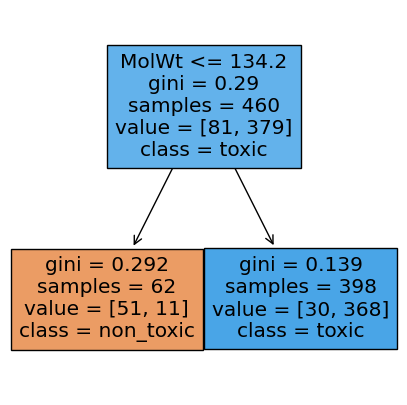
Now, let’s visualize the rule. The tree plot below shows the root node with its split, the Gini impurity at each node, the sample counts, and the class distribution. Filled colors hint at the majority class in each leaf.

# Visualize stump
plt.figure(figsize=(5,5))
plot_tree(stump, feature_names=feat_names, class_names=["non_toxic","toxic"], filled=True, impurity=True)
plt.show()

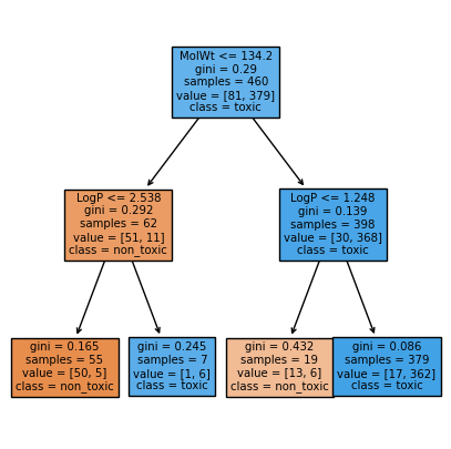
We can also visualize max_depth=2 to see the difference:

stump2 = DecisionTreeClassifier(max_depth=2, criterion="gini", random_state=0)
stump2.fit(X_train, y_train)

plt.figure(figsize=(5,5))
plot_tree(stump2, feature_names=feat_names, class_names=["non_toxic","toxic"], filled=True, impurity=True)
plt.show()

---

1.4 Grow deeper and control overfitting

Trees can fit noise if we let them grow without limits. We control growth using a few simple knobs.

• max_depth: limit the number of levels

• min_samples_split: a node needs at least this many samples to split

• min_samples_leaf: each leaf must have at least this many samples

def fit_eval_tree(max_depth=None, min_leaf=1):
    clf = DecisionTreeClassifier(
        max_depth=max_depth, min_samples_leaf=min_leaf, random_state=0
    )
    clf.fit(X_train, y_train)
    acc = accuracy_score(y_test, clf.predict(X_test))
    return clf, acc

depths = [1, 2, 3, 4, 5, None]  # None means grow until pure or exhausted
scores = []
for d in depths:
    _, acc = fit_eval_tree(max_depth=d, min_leaf=3)
    scores.append(acc)

pd.DataFrame({"max_depth": [str(d) for d in depths], "Accuracy": np.round(scores,3)})

	max_depth	Accuracy
0	1	0.922
1	2	0.957
2	3	0.948
3	4	0.948
4	5	0.948
5	None	0.930

Here, we hold min_samples_leaf = 3 and vary max_depth. This shows the classic underfit to overfit trend.

plt.plot([str(d) for d in depths], scores, marker="o")
plt.xlabel("max_depth")
plt.ylabel("Accuracy (test)")
plt.title("Tree depth vs test accuracy")
plt.grid(True)
plt.show()

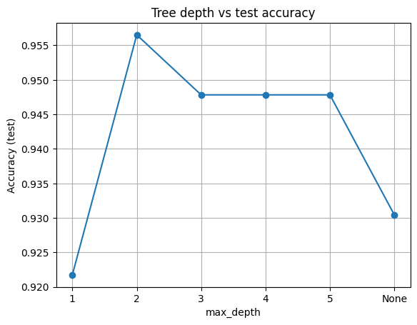
Takeaway

Shallow trees underfit. Very deep trees often overfit. Start small, add depth only if validation improves.

Now, let’s try sweep leaf size at several depths.

We will try a small grid. This lets you see both knobs together.

def fit_acc_leaves(max_depth=None, min_leaf=1):
    clf = DecisionTreeClassifier(
        max_depth=max_depth, min_samples_leaf=min_leaf, random_state=0
    )
    clf.fit(X_train, y_train)
    acc_test = accuracy_score(y_test, clf.predict(X_test))
    n_leaves = clf.get_n_leaves()  # simple and reliable
    return acc_test, n_leaves

leaf_sizes = [1, 3, 5, 10, 20]
depths = [1, 2, 3, 4, 5, None]

rows = []
for leaf in leaf_sizes:
    for d in depths:
        acc, leaves = fit_acc_leaves(max_depth=d, min_leaf=leaf)
        rows.append({
            "min_samples_leaf": leaf,
            "max_depth": str(d),
            "acc_test": acc,
            "n_leaves": leaves
        })

df_grid = pd.DataFrame(rows).sort_values(
    ["min_samples_leaf","max_depth"]
).reset_index(drop=True)
df_grid

	min_samples_leaf	max_depth	acc_test	n_leaves
0	1	1	0.921739	2
1	1	2	0.956522	4
2	1	3	0.947826	8
3	1	4	0.947826	13
4	1	5	0.947826	18
5	1	None	0.921739	34
6	3	1	0.921739	2
7	3	2	0.956522	4
8	3	3	0.947826	8
9	3	4	0.947826	12
10	3	5	0.947826	17
11	3	None	0.930435	25
12	5	1	0.921739	2
13	5	2	0.956522	4
14	5	3	0.939130	7
15	5	4	0.939130	12
16	5	5	0.939130	15
17	5	None	0.921739	20
18	10	1	0.921739	2
19	10	2	0.956522	4
20	10	3	0.956522	6
21	10	4	0.956522	9
22	10	5	0.947826	11
23	10	None	0.947826	13
24	20	1	0.921739	2
25	20	2	0.939130	4
26	20	3	0.939130	6
27	20	4	0.939130	8
28	20	5	0.939130	9
29	20	None	0.939130	9

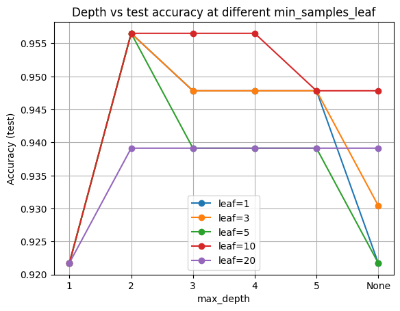
Now, we plot test accuracy vs depth for each leaf size.

Higher min_samples_leaf tends to smooth the curves and reduce the train minus test gap.

Hyperparamter

Higher min_samples_leaf tends to smooth the curves and reduce the train minus test gap.

plt.figure()
for leaf in leaf_sizes:
    sub = df_grid[df_grid["min_samples_leaf"]==leaf]
    plt.plot(sub["max_depth"], sub["acc_test"], marker="o", label=f"leaf={leaf}")
plt.xlabel("max_depth")
plt.ylabel("Accuracy (test)")
plt.title("Depth vs test accuracy at different min_samples_leaf")
plt.grid(True)
plt.legend()
plt.show()

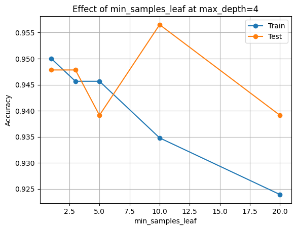
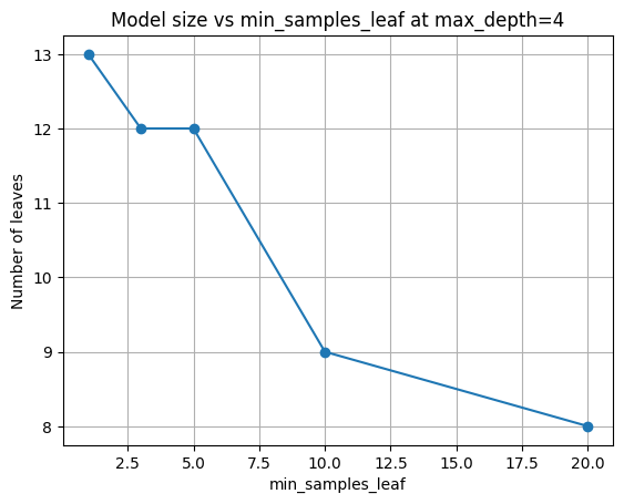
Finally, let’s look at what happen if we fix depth and vary leaf size:

Pick a moderate depth (4), then look at how leaf size alone affects accuracy and model size.

fixed_depth = 4
rows = []
for leaf in leaf_sizes:
    clf = DecisionTreeClassifier(
        max_depth=fixed_depth, min_samples_leaf=leaf, random_state=0
    ).fit(X_train, y_train)

    rows.append({
        "min_samples_leaf": leaf,
        "acc_train": accuracy_score(y_train, clf.predict(X_train)),
        "acc_test":  accuracy_score(y_test,  clf.predict(X_test)),
        "n_nodes":   clf.tree_.node_count,
        "n_leaves":  clf.get_n_leaves(),
    })

df_leaf = pd.DataFrame(rows).sort_values("min_samples_leaf").reset_index(drop=True)
df_leaf[["min_samples_leaf","acc_train","acc_test","n_nodes","n_leaves"]]

	min_samples_leaf	acc_train	acc_test	n_nodes	n_leaves
0	1	0.950000	0.947826	25	13
1	3	0.945652	0.947826	23	12
2	5	0.945652	0.939130	23	12
3	10	0.934783	0.956522	17	9
4	20	0.923913	0.939130	15	8

plt.figure()
plt.plot(df_leaf["min_samples_leaf"], df_leaf["acc_train"], marker="o", label="Train")
plt.plot(df_leaf["min_samples_leaf"], df_leaf["acc_test"],  marker="o", label="Test")
plt.xlabel("min_samples_leaf")
plt.ylabel("Accuracy")
plt.title(f"Effect of min_samples_leaf at max_depth={fixed_depth}")
plt.grid(True)
plt.legend()
plt.show()

plt.figure()
plt.plot(df_leaf["min_samples_leaf"], df_leaf["n_leaves"], marker="o")
plt.xlabel("min_samples_leaf")
plt.ylabel("Number of leaves")
plt.title(f"Model size vs min_samples_leaf at max_depth={fixed_depth}")
plt.grid(True)
plt.show()

Underfitting vs. Overfitting

Higher min_samples_leaf tends to smooth the curves and reduce the train minus test gap.

• Underfitting
  Happens when the model is too simple to capture meaningful patterns.
  Signs:

  • Both training and test accuracy are low.

  • The decision boundary looks crude.

  • Increasing model capacity (like depth) improves results.

• Overfitting
  Happens when the model is too complex and memorizes noise in the training set.
  Signs:

  • Training accuracy is very high (often near 100%).

  • Test accuracy lags behind.

  • Model has many small leaves with very few samples.

  • Predictions fluctuate wildly for minor changes in input.

The goal is good generalization: high performance on unseen data, not just on the training set.

---

1.5 Model-based importance: Gini importance

As we learned in lecture 6, ML models not only make predictions but also provide insight into which features were most useful.

There are two main ways we can measure this: Gini importance (model-based) and permutation importance (data-based). Both give us different perspectives on feature relevance.

When fitting a tree, each split reduces impurity (measured by Gini or entropy). A feature’s importance is computed as:

• The total decrease in impurity that results from splits on that feature

• Normalized so that all features sum to 1

This is fast and built-in, but it reflects how the model used the features during training. It may overstate the importance of high-cardinality or correlated features.

tree_clf = DecisionTreeClassifier(max_depth=4, min_samples_leaf=3, random_state=0).fit(X_train, y_train)

imp = pd.Series(tree_clf.feature_importances_, index=feat_names).sort_values(ascending=False)
imp

MolWt       0.601322
LogP        0.291825
TPSA        0.085734
NumRings    0.021119
dtype: float64

imp.plot(kind="barh")
plt.title("Gini importance (tree)")
plt.gca().invert_yaxis()
plt.show()

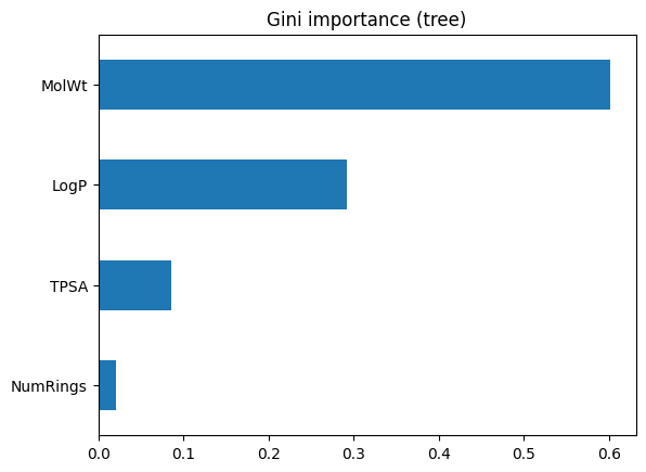
This bar chart above ranks features by how much they reduced impurity in the training process. The top feature is the one the tree found most useful for splitting. However, keep in mind this is internal to the model and may not reflect true predictive power on unseen data.

---

1.6 Data-based importance: Permutation importance

Permutation importance takes a different approach. Instead of looking inside the model, it asks: What happens if I scramble a feature’s values on the test set? If accuracy drops, that feature was important. If accuracy stays the same, the model did not really depend on it.

Steps:

1. Shuffle one feature column at a time in the test set.

2. Measure the drop in accuracy.

3. Repeat many times and average to reduce randomness.

perm = permutation_importance(
    tree_clf, X_test, y_test, scoring="accuracy", n_repeats=20, random_state=0
)
perm_ser = pd.Series(perm.importances_mean, index=feat_names).sort_values()
perm_ser.plot(kind="barh")
plt.title("Permutation importance (test)")
plt.show()

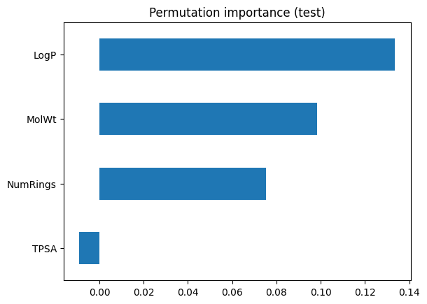
Here, the bars show how much accuracy falls when each feature is disrupted. This provides a more honest reflection of predictive value on unseen data. Features that looked strong in Gini importance may shrink here if they were just splitting on quirks of the training set.

⏰ Exercise 1.6

Compute permutation importance on the test set with scoring="roc_auc" and again with scoring="f1". Any difference?

When we compare the two methods, we will see the difference is: Gini importance (tree-based):

Easy to compute. Biased toward features with many possible split points. Reflects training behavior, not necessarily generalization.

Permutation importance (test-based):

More computationally expensive (requires multiple shuffles). Directly tied to model performance on new data. Can reveal when the model “thought” a feature was important but it doesn’t hold up in practice.

---

2. Regression trees on Melting Point

So far we used trees for classification. Now we switch to a regression target: the melting point of molecules. The mechanics are similar, but instead of predicting a discrete class, the tree predicts a continuous value.

df_reg = df[["MolWt", "LogP", "TPSA", "NumRings", "Melting Point"]].dropna()
Xr = df_reg[["MolWt", "LogP", "TPSA", "NumRings"]]
yr = df_reg["Melting Point"]

Xr_train, Xr_test, yr_train, yr_test = train_test_split(
    Xr, yr, test_size=0.2, random_state=42
)

Xr_train.head(2), yr_train.head(3)

(       MolWt    LogP  TPSA  NumRings
 68   226.703  3.6870  26.3       1.0
 231  282.295  2.5255  52.6       3.0,
 68     152.1
 231    169.4
 63     247.3
 Name: Melting Point, dtype: float64)

Just like before, we can grow a stump (·max_depth=1·) to see a single split. Instead of class impurity, the split criterion is reduction in variance of the target.

reg_stump = DecisionTreeRegressor(max_depth=1, random_state=0)
reg_stump.fit(Xr_train, yr_train)
print("Root feature:", Xr_train.columns[reg_stump.tree_.feature[0]])
print("Root threshold:", reg_stump.tree_.threshold[0])

Root feature: MolWt
Root threshold: 245.61299896240234

What can we learn from Root Feature output?

This tells us the first cut is on MolW. Samples with weight below ~246 g/mol are grouped separately from heavier ones.

Let’s vary max_depth and track R² on the test set. Remember:

R² = 1 means perfect prediction, R² = 0 means the model is no better than the mean.

Below, we pick depth = 3, leaf size = 5. This is a good trade-off.

# Evaluate shallow vs deeper
depths = [1, 2, 3, 4, 6, 8, None]
r2s = []
for d in depths:
    reg = DecisionTreeRegressor(max_depth=d, min_samples_leaf=5, random_state=0).fit(Xr_train, yr_train)
    yhat = reg.predict(Xr_test)
    r2s.append(r2_score(yr_test, yhat))

pd.DataFrame({"max_depth": [str(d) for d in depths], "R2_test": np.round(r2s,3)})

	max_depth	R2_test
0	1	0.398
1	2	0.659
2	3	0.810
3	4	0.809
4	6	0.777
5	8	0.765
6	None	0.761

plt.plot([str(d) for d in depths], r2s, marker="o")
plt.xlabel("max_depth")
plt.ylabel("R2 on test")
plt.title("Regression tree depth vs R2")
plt.grid(True)
plt.show()

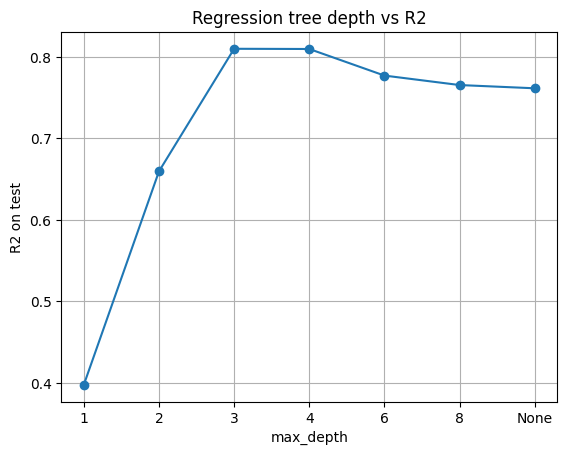
This mirrors the classification case: shallow trees underfit, very deep trees overfit.

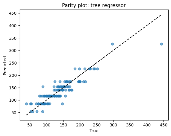
Points close to the dashed line = good predictions. Scatter away from the line = errors. Here, predictions track well but show some spread at high melting points.

# Diagnostics for a chosen depth
reg = DecisionTreeRegressor(max_depth=3, min_samples_leaf=5, random_state=0).fit(Xr_train, yr_train)
yhat = reg.predict(Xr_test)

print(f"MSE={mean_squared_error(yr_test, yhat):.3f}")
print(f"MAE={mean_absolute_error(yr_test, yhat):.3f}")
print(f"R2={r2_score(yr_test, yhat):.3f}")

# Parity
plt.scatter(yr_test, yhat, alpha=0.6)
lims = [min(yr_test.min(), yhat.min()), max(yr_test.max(), yhat.max())]
plt.plot(lims, lims, "k--")
plt.xlabel("True")
plt.ylabel("Predicted")
plt.title("Parity plot: tree regressor")
plt.show()

# Residuals
res = yr_test - yhat
plt.scatter(yhat, res, alpha=0.6)
plt.axhline(0, color="k", linestyle="--")
plt.xlabel("Predicted")
plt.ylabel("Residual")
plt.title("Residual plot: tree regressor")
plt.show()

MSE=566.158
MAE=17.574
R2=0.810

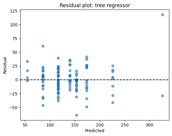
Similar to the example we see on the linear regression, residuals (true – predicted) should scatter around zero. If you see patterns (e.g., always underpredicting high values), the model may be biased. Here, residuals are fairly centered but not perfectly homoscedastic.

⏰ Exercise 2

Train two regression trees with max_depth=6 using min_samples_leaf=5. Report R² and MAE for both and show the two parity plots.

# Visualize a small regression tree
plt.figure(figsize=(15,10))
plot_tree(reg, feature_names=Xr_train.columns, filled=True, impurity=True, rounded=True, proportion=False)
plt.show()

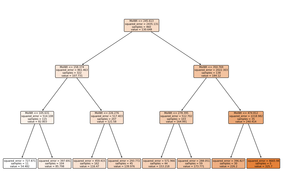
Regression tree vs classifier tree

A regression tree is structured the same as a classifier tree, but each leaf stores an average target value instead of a class distribution.

---

3. Random Forest: bagging many trees

Decision trees are intuitive but unstable: a small change in data can produce a very different tree. To make trees more reliable and accurate, we use ensembles — groups of models working together. The most widely used ensemble of trees is the Random Forest.

Eseentially, a random forest grows many decision trees, each trained on a slightly different view of the data, and then combines their predictions:

• Bootstrap sampling (bagging):
  Each tree sees a different random subset of the training rows, sampled with replacement. About one-third of rows are left out for that tree (these are the out-of-bag samples).

• Feature subsampling:
  At each split, the tree does not see all features — only a random subset, controlled by max_features. This prevents trees from always picking the same strong predictor and encourages diversity.

Each tree may be a weak learner, but when you average many diverse trees, the variance cancels out. This makes forests much more stable and accurate than single trees, especially on noisy data.

---

Here are some helpful aspect of forests:

• Single deep tree → low bias, high variance (overfit easily).

• Forest of many deep trees → still low bias, but variance shrinks when you average.

• Built-in validation: out-of-bag samples allow you to estimate performance without needing a separate validation set.

In practice, random forests are a strong default: robust, interpretable at the feature level, and requiring little parameter tuning.

3.1 Classification forest on toxicity

We now build a forest to classify molecules as toxic vs non-toxic.
We set:

• n_estimators=300: number of trees.

• max_features="sqrt": common heuristic for classification.

• min_samples_leaf=3: prevent leaves with only 1 or 2 samples.

rf_clf = RandomForestClassifier(
    n_estimators=300,
    max_depth=None,
    min_samples_leaf=3,
    max_features="sqrt",
    oob_score=True,          # enable OOB estimation, if you dont specify, the default RF will not give you oob
    random_state=0,
)
rf_clf.fit(X_train, y_train)

print("OOB score:", rf_clf.oob_score_)
acc = accuracy_score(y_test, rf_clf.predict(X_test))
print("Test accuracy:", acc)

OOB score: 0.9282608695652174
Test accuracy: 0.9478260869565217

Here, Out-of-Bag (OOB) Score gives an internal validation accuracy, while test accuracy confirms performance on held-out data.

How the OOB score is calculated

1. For each training point, collect predictions only from the trees that did not see that point during training (its out-of-bag trees).

2. Aggregate those predictions (majority vote for classification, mean for regression).

3. Compare aggregated predictions against the true labels.

4. The accuracy (or R² for regression) across all training samples is the OOB score.

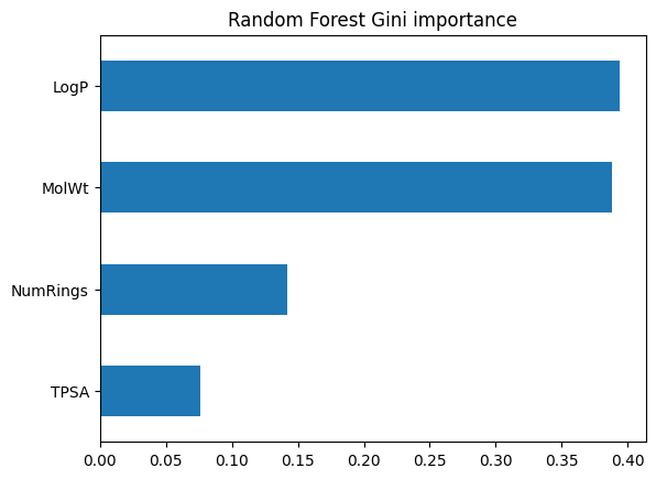
Forests average over many trees, so feature importance is more reliable than from a single tree. We can view both Gini importance and permutation importance.

imp_rf = pd.Series(rf_clf.feature_importances_, index=feat_names).sort_values()
imp_rf.plot(kind="barh")
plt.title("Random Forest Gini importance")
plt.show()

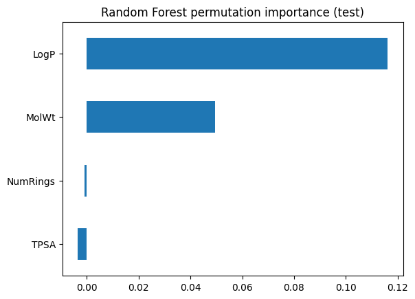
perm_rf = permutation_importance(rf_clf, X_test, y_test, scoring="accuracy", n_repeats=20, random_state=0)
pd.Series(perm_rf.importances_mean, index=feat_names).sort_values().plot(kind="barh")
plt.title("Random Forest permutation importance (test)")
plt.show()

3.2 Regression forest on Melting Point

Next we apply the same idea for regression. The forest predicts a continuous value (melting point) by averaging predictions from many regression trees.

# Reload mp dataset so X and y are updated
df_reg_mp = df[["MolWt", "LogP", "TPSA", "NumRings", "Melting Point"]].dropna()
Xr_mp = df_reg_mp[["MolWt", "LogP", "TPSA", "NumRings"]]
yr_mp = df_reg_mp["Melting Point"]

Xr_mp_train, Xr_mp_test, yr_mp_train, yr_mp_test = train_test_split(
    Xr_mp, yr_mp, test_size=0.2, random_state=0
)

# Random Forest (mp-specific)
rf_reg_mp = RandomForestRegressor(
    n_estimators=400,
    max_depth=None,
    max_features="sqrt",
    random_state=0,
)
rf_reg_mp.fit(Xr_mp_train, yr_mp_train)

yhat_rf_mp = rf_reg_mp.predict(Xr_mp_test)
print("Random Forest (mp)")
print(f"Test R2: {r2_score(yr_mp_test, yhat_rf_mp):.3f}")
print(f"Test MAE: {mean_absolute_error(yr_mp_test, yhat_rf_mp):.3f}")

# Lasso baseline (mp-specific), fixed alpha=0.1 with scaling
lasso_reg_mp = Lasso(alpha=0.1, random_state=0, max_iter=500)
lasso_reg_mp.fit(Xr_mp_train, yr_mp_train)

yhat_lasso_mp = lasso_reg_mp.predict(Xr_mp_test)
print("\nLasso (mp, alpha=0.1)")
print(f"Test R2: {r2_score(yr_mp_test, yhat_lasso_mp):.3f}")
print(f"Test MAE: {mean_absolute_error(yr_mp_test, yhat_lasso_mp):.3f}")

Random Forest (mp)
Test R2: 0.730
Test MAE: 18.062

Lasso (mp, alpha=0.1)
Test R2: 0.771
Test MAE: 16.952

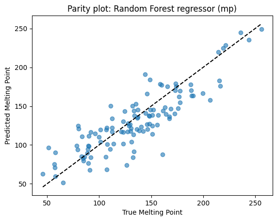
Parity and feature importance plots help check performance.

# --- Parity plot for mp RF ---
plt.scatter(yr_mp_test, yhat_rf_mp, alpha=0.6)
lims = [min(yr_mp_test.min(), yhat_rf_mp.min()), max(yr_mp_test.max(), yhat_rf_mp.max())]
plt.plot(lims, lims, "k--")
plt.xlabel("True Melting Point")
plt.ylabel("Predicted Melting Point")
plt.title("Parity plot: Random Forest regressor (mp)")
plt.show()

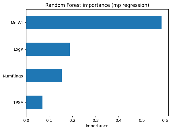
# --- Feature importance for mp RF ---
pd.Series(rf_reg_mp.feature_importances_, index=Xr_mp_train.columns) \
    .sort_values() \
    .plot(kind="barh")

plt.title("Random Forest importance (mp regression)")
plt.xlabel("Importance")
plt.show()

---

4. Ensembles

Ensembles combine multiple models to improve stability and accuracy. Here we expand on trees with forests, simple averaging, voting, and boosting, and add visual comparisons to show their differences.

---

4.1 Experiment: single tree vs random forest

We repeat training several times with different random seeds for the train/test split. For each split:

• Fit a single unpruned tree.

• Fit a random forest with 300 trees.

• Record the test R² for both.

splits = [1, 7, 21, 42, 77]
rows = []
for seed in splits:
    X_tr, X_te, y_tr, y_te = train_test_split(Xr, yr, test_size=0.2, random_state=seed)
    t = DecisionTreeRegressor(max_depth=None, min_samples_leaf=3, random_state=seed).fit(X_tr, y_tr)
    f = RandomForestRegressor(n_estimators=300, min_samples_leaf=3, random_state=seed).fit(X_tr, y_tr)
    r2_t = r2_score(y_te, t.predict(X_te))
    r2_f = r2_score(y_te, f.predict(X_te))
    rows.append({"seed": seed, "Tree_R2": r2_t, "Forest_R2": r2_f})

df_cmp = pd.DataFrame(rows).round(3)
df_cmp

	seed	Tree_R2	Forest_R2
0	1	0.710	0.801
1	7	0.670	0.794
2	21	0.771	0.792
3	42	0.747	0.824
4	77	0.768	0.814

plt.plot(df_cmp["seed"], df_cmp["Tree_R2"], "o-", label="Tree")
plt.plot(df_cmp["seed"], df_cmp["Forest_R2"], "o-", label="Forest")
plt.xlabel("random_state")
plt.ylabel("R2 on test")
plt.title("Stability across splits")
plt.legend()
plt.grid(True)
plt.show()

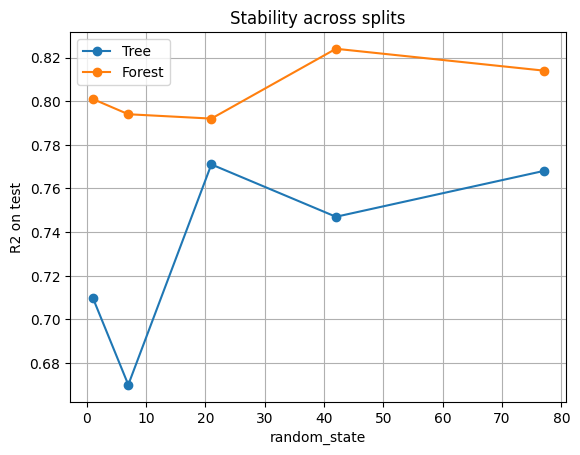
Why forests are often a safe and strong default model

• Single tree: R² jumps up and down depending on the seed. Sometimes the tree performs decently, sometimes it collapses.

• Random forest: R² is consistently higher and more stable. By averaging across 300 trees trained on different bootstrap samples and feature subsets, the forest cancels out randomness.
  Forests trade a bit of interpretability for much more reliability.

---

4.2 Simple Ensembles by Model Averaging

Random forests are powerful, but ensembling can be simpler. Even just averaging two different models can improve performance.

from sklearn.linear_model import LinearRegression

tree = DecisionTreeRegressor(max_depth=4).fit(Xr_train, yr_train)
lin  = LinearRegression().fit(Xr_train, yr_train)

pred_tree = tree.predict(Xr_test)
pred_lin  = lin.predict(Xr_test)
pred_avg = (pred_tree + pred_lin) / 2.0

df_avg = pd.DataFrame({
    "True": yr_test,
    "Tree": pred_tree,
    "Linear": pred_lin,
    "Average": pred_avg
}).head(10)
df_avg

	True	Tree	Linear	Average
153	130.4	121.423000	116.903234	119.163117
118	91.5	94.747826	93.587419	94.167622
245	158.9	167.670370	165.901961	166.786166
408	75.0	83.256790	80.402677	81.829734
278	176.1	136.764865	138.856393	137.810629
185	123.8	108.482258	109.010862	108.746560
234	154.3	159.203571	153.651410	156.427490
29	200.3	178.918750	184.189243	181.553997
82	88.1	83.256790	87.838467	85.547628
158	82.6	121.423000	119.893550	120.658275

print("Tree R2:", r2_score(yr_test, pred_tree))
print("Linear R2:", r2_score(yr_test, pred_lin))
print("Averaged R2:", r2_score(yr_test, pred_avg))

Tree R2: 0.8514902671757174
Linear R2: 0.8741026174988968
Averaged R2: 0.869699219889096

plt.scatter(yr_test, pred_tree, alpha=0.5, label="Tree")
plt.scatter(yr_test, pred_lin, alpha=0.5, label="Linear")
plt.scatter(yr_test, pred_avg, alpha=0.5, label="Average")
lims = [min(yr_test.min(), pred_tree.min(), pred_lin.min()), max(yr_test.max(), pred_tree.max(), pred_lin.max())]
plt.plot(lims, lims, "k--")
plt.xlabel("True")
plt.ylabel("Predicted")
plt.title("Parity plot: Tree vs Linear vs Average")
plt.legend()
plt.show()

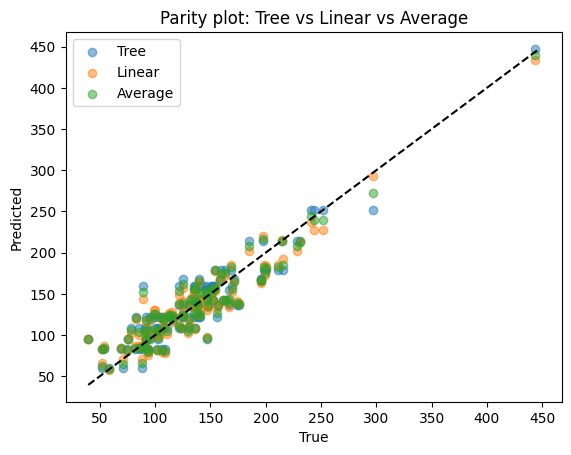
Difference

• Tree: captures nonlinear shapes but may overfit.

• Linear: very stable but may underfit.

• Average: balances the two, smoother than tree, more flexible than linear regression.

---

4.3 Simple Ensembles by Voting

Voting is most common for classification. Each model votes for a class.

• Hard voting: majority wins.

• Soft voting: average predicted probabilities.

from sklearn.ensemble import VotingClassifier
from sklearn.linear_model import LogisticRegression


vote_clf_soft = VotingClassifier(
    estimators=[
        ("lr", LogisticRegression(max_iter=500, random_state=0)),
        ("lr2", LogisticRegression(max_iter=11000, random_state=0)),
        ("rf", RandomForestClassifier(n_estimators=100, random_state=0)),
        ("rf2", RandomForestClassifier(n_estimators=30, random_state=0))
    ],
    voting="soft"
).fit(X_train, y_train)

print("Soft Voting classifier accuracy:", accuracy_score(y_test, vote_clf_soft.predict(X_test)))


vote_clf_hard = VotingClassifier(
    estimators=[
        ("lr", LogisticRegression(max_iter=500, random_state=0)),
        ("lr2", LogisticRegression(max_iter=11000, random_state=0)),
        ("rf", RandomForestClassifier(n_estimators=100, random_state=0)),
        ("rf2", RandomForestClassifier(n_estimators=30, random_state=0))
    ],
    voting="hard"
).fit(X_train, y_train)

print("Hard Voting classifier accuracy:", accuracy_score(y_test, vote_clf_hard.predict(X_test)))

Soft Voting classifier accuracy: 0.9652173913043478
Hard Voting classifier accuracy: 0.9565217391304348

Compare voting against individual models:

acc_lr = accuracy_score(y_test, LogisticRegression(max_iter=500, random_state=0).fit(X_train,y_train).predict(X_test))
acc_rf  = accuracy_score(y_test, RandomForestClassifier(n_estimators=100, random_state=0).fit(X_train,y_train).predict(X_test))

pd.DataFrame({
    "Model": ["LogReg", "RandomForest", "Voting-Hard", "Voting-Soft"],
    "Accuracy": [acc_lr, acc_rf, accuracy_score(y_test, vote_clf_hard.predict(X_test)), accuracy_score(y_test, vote_clf_soft.predict(X_test))]
})

	Model	Accuracy
0	LogReg	0.956522
1	RandomForest	0.939130
2	Voting-Hard	0.956522
3	Voting-Soft	0.965217

Difference

• Individual models: Logistic regression handles linear patterns, SVM picks margins, random forest handles nonlinear rules.

• Voting ensemble: combines their strengths, reducing the chance of one weak model dominating.

---

4.4 (Optional Topic) Boosting: a different ensemble structure

Boosting is sequential: each tree corrects the mistakes of the last. Sometimes it can be stronger than bagging, but needs careful tuning.

from sklearn.ensemble import GradientBoostingRegressor
from sklearn.metrics import mean_absolute_error

gb_reg = GradientBoostingRegressor(
    n_estimators=300,
    learning_rate=0.05,
    max_depth=3,
    random_state=0
).fit(Xr_train, yr_train)

yhat_gb = gb_reg.predict(Xr_test)
print(f"Gradient Boosting R2: {r2_score(yr_test, yhat_gb):.3f}")
print(f"Gradient Boosting MAE: {mean_absolute_error(yr_test, yhat_gb):.2f}")

Gradient Boosting R2: 0.856
Gradient Boosting MAE: 16.17

Compare Random Forest vs Gradient Boosting directly:

rf_reg = RandomForestRegressor(n_estimators=300, min_samples_leaf=3, random_state=0).fit(Xr_train, yr_train)
yhat_rf = rf_reg.predict(Xr_test)

pd.DataFrame({
    "Model": ["RandomForest", "GradientBoosting"],
    "R2": [r2_score(yr_test, yhat_rf), r2_score(yr_test, yhat_gb)],
    "MAE": [mean_absolute_error(yr_test, yhat_rf), mean_absolute_error(yr_test, yhat_gb)]
}).round(3)

	Model	R2	MAE
0	RandomForest	0.826	16.777
1	GradientBoosting	0.856	16.172

plt.scatter(yr_test, yhat_rf, alpha=0.5, label="RandomForest")
plt.scatter(yr_test, yhat_gb, alpha=0.5, label="GradientBoosting")
lims = [min(yr_test.min(), yhat_rf.min(), yhat_gb.min()), max(yr_test.max(), yhat_rf.max(), yhat_gb.max())]
plt.plot(lims, lims, "k--")
plt.xlabel("True")
plt.ylabel("Predicted")
plt.title("Parity plot: RF vs GB")
plt.legend()
plt.show()

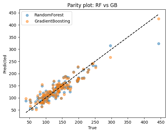
Compare

• Random forest: reduces variance by averaging many deep trees. Stable and easy to tune.

• Boosting: reduces bias by sequentially correcting mistakes. Often achieves higher accuracy but requires careful parameter tuning.

---

5. End-to-end recipe for random forest

Now, let’s put everything we learn for trees and forests together. Below is a standard workflow for toxicity with a forest. Similar to what we learned from last lecture but handled with RF model.

# 1) Data
X = df_clf[["MolWt", "LogP", "TPSA", "NumRings"]]
y = df_clf["Toxicity"].str.lower().map(label_map).astype(int)

X_train, X_test, y_train, y_test = train_test_split(
    X, y, test_size=0.2, random_state=15, stratify=y
)

# 2) Model
rf = RandomForestClassifier(
    n_estimators=400, max_depth=None, max_features="sqrt",
    min_samples_leaf=3, oob_score=True, random_state=15
).fit(X_train, y_train)

# 3) Evaluate
y_hat = rf.predict(X_test)
y_proba = rf.predict_proba(X_test)[:,1]
print(f"OOB score: {rf.oob_score_:.3f}")
print(f"Accuracy: {accuracy_score(y_test, y_hat):.3f}")
print(f"AUC: {roc_auc_score(y_test, y_proba):.3f}")

OOB score: 0.939
Accuracy: 0.922
AUC: 0.955

In addition to just fit model with trainset using either default or pre-defined n_estimators and max_depth, as we learned from last lecture, a more solid way will be search/tune for possible combinations of hyperparamters during the cross validation.

As you see below, it will take longer time to run (since it surveys 2 x 2 x 2 = 8 combinations in total and is more computationally expensive) but result in better performance.

from sklearn.model_selection import KFold, GridSearchCV
from sklearn.ensemble import RandomForestClassifier
from sklearn.metrics import accuracy_score, roc_auc_score, classification_report

# Data
X = df_clf[["MolWt", "LogP", "TPSA", "NumRings"]]
y = df_clf["Toxicity"].str.lower().map(label_map).astype(int)

X_train, X_test, y_train, y_test = train_test_split(
    X, y, test_size=0.2, random_state=42, stratify=y
)

# KFold CV search
cv = KFold(n_splits=5, shuffle=True, random_state=15)

rf = RandomForestClassifier(random_state=15)
param_grid = {
    "n_estimators": [50, 500],
    "max_depth": [None, 20],
    "min_samples_leaf": [1, 3],
}

gs = GridSearchCV(
    estimator=rf,
    param_grid=param_grid,
    scoring="roc_auc",
    cv=cv,
    refit=True,
)

gs.fit(X_train, y_train)
best_rf = gs.best_estimator_
print("Best params:", gs.best_params_)
print(f"Best CV AUC: {gs.best_score_:.3f}")

# Test evaluation
y_hat = best_rf.predict(X_test)
y_proba = best_rf.predict_proba(X_test)[:, 1]
print(f"Accuracy: {accuracy_score(y_test, y_hat):.3f}")
print(f"AUC: {roc_auc_score(y_test, y_proba):.3f}")
print(classification_report(y_test, y_hat, digits=3))

Best params: {'max_depth': None, 'min_samples_leaf': 3, 'n_estimators': 500}
Best CV AUC: 0.972
Accuracy: 0.948
AUC: 0.982
              precision    recall  f1-score   support

           0      0.850     0.850     0.850        20
           1      0.968     0.968     0.968        95

    accuracy                          0.948       115
   macro avg      0.909     0.909     0.909       115
weighted avg      0.948     0.948     0.948       115

Additional plots demonstrating the performance:

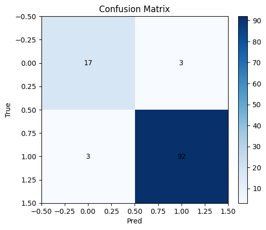
# Confusion matrix and ROC
cm = confusion_matrix(y_test, y_hat)
plt.imshow(cm, cmap="Blues"); plt.title("Confusion Matrix"); plt.xlabel("Pred"); plt.ylabel("True")
for i in range(2):
    for j in range(2):
        plt.text(j, i, cm[i,j], ha="center", va="center")
plt.colorbar(fraction=0.046, pad=0.04)
plt.show()

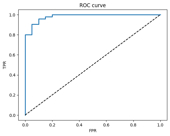
fpr, tpr, thr = roc_curve(y_test, y_proba)
plt.plot(fpr, tpr, lw=2); plt.plot([0,1],[0,1],"k--")
plt.xlabel("FPR"); plt.ylabel("TPR"); plt.title("ROC curve")
plt.show()

---

6. Quick reference

Common options

• DecisionTreeClassifier/Regressor: max_depth, min_samples_leaf, min_samples_split, criterion, random_state

• RandomForestClassifier/Regressor: add n_estimators, max_features, oob_score, n_jobs

• Use feature_importances_ for built-in importance and permutation_importance for model-agnostic view

When to use

• Tree: simple rules, quick to interpret on small depth

• Forest: stronger accuracy, more stable, less sensitive to a single split

---

7. In-class activities

7.1 Tree vs Forest on log-solubility

• Create y_log = log10(Solubility_mol_per_L + 1e-6)

• Use features [MolWt, LogP, TPSA, NumRings]

• Train a DecisionTreeRegressor(max_depth=4, min_samples_leaf=5) and a RandomForestRegressor(n_estimators=300, min_samples_leaf=5)

• Report test R2 for both and draw both parity plots

# TO DO

7.2 Pruning with min_samples_leaf

• Fix max_depth=None for DecisionTreeClassifier on toxicity

• Sweep min_samples_leaf in [1, 2, 3, 5, 8, 12, 20]

• Plot test accuracy vs min_samples_leaf

# TO DO

7.3 Toxicity prediction

• Train a DecisionTreeClassifier(max_depth=2) on toxicity

• Use plot_tree to draw it and write down the two split rules in plain language

Optional:

• Train RandomForestClassifier with oob_score=True on toxicity

• Compare OOB score to test accuracy over seeds [0, 7, 21, 42]

# TO DO

7.4 Feature importance agreement

• On melting point, compute forest feature_importances_ and permutation_importance

• Plot both and comment where they agree or disagree

# TO DO

7.5 Hyperparameter search with cross validation

Use GridSearchCV on RandomForestClassifier for toxicity

Split once into train and test as usual, but perform 5-fold CV only on the training fold

Search over:

n_estimators: [200, 400]

max_depth: [None, 6, 10]

min_samples_leaf: [1, 2, 3, 5]

max_features: [“sqrt”, 0.8]

Use scoring="roc_auc" for the CV score

After the search, refit the best model on the full training data

Report: **best params, CV AUC, test Accuracy and test AUC

Plot ROC curve for the final model

Hint: This may take more than 30 s to run since it searches for quite a few hyperparameters

# TO DO

---

8. Solutions

Q1

Goal: predict log-solubility and compare a small tree to a forest.

# Create target: log10(solubility + 1e-6) to avoid log(0)
# If your dataframe already has a numeric solubility column named 'Solubility_mol_per_L', reuse it.
df_sol = df.copy()
df_sol["y_log"] = np.log10(df_sol["Solubility_mol_per_L"] + 1e-6)

Xs = df_sol[["MolWt", "LogP", "TPSA", "NumRings"]].dropna()
ys = df_sol.loc[Xs.index, "y_log"]

Xs_train, Xs_test, ys_train, ys_test = train_test_split(
    Xs, ys, test_size=0.2, random_state=42
)

# Models
tree_sol = DecisionTreeRegressor(max_depth=4, min_samples_leaf=5, random_state=0).fit(Xs_train, ys_train)
rf_sol   = RandomForestRegressor(n_estimators=300, min_samples_leaf=5, random_state=0).fit(Xs_train, ys_train)

# Scores
yhat_tree = tree_sol.predict(Xs_test)
yhat_rf   = rf_sol.predict(Xs_test)

print(f"Tree R2:   {r2_score(ys_test, yhat_tree):.3f}")
print(f"Forest R2: {r2_score(ys_test, yhat_rf):.3f}")

Tree R2:   0.918
Forest R2: 0.947

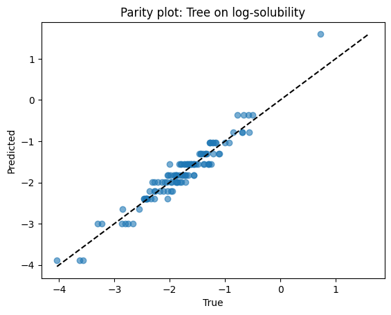
Parity plots for both models.

# Parity for tree
plt.scatter(ys_test, yhat_tree, alpha=0.6)
lims = [min(ys_test.min(), yhat_tree.min()), max(ys_test.max(), yhat_tree.max())]
plt.plot(lims, lims, "k--")
plt.xlabel("True")
plt.ylabel("Predicted")
plt.title("Parity plot: Tree on log-solubility")
plt.show()

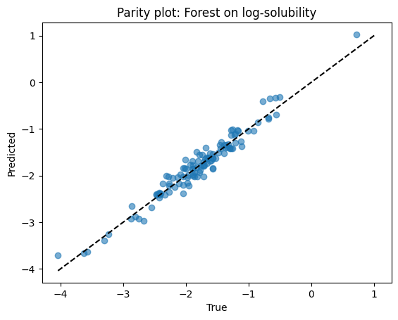
# Parity for forest
plt.scatter(ys_test, yhat_rf, alpha=0.6)
lims = [min(ys_test.min(), yhat_rf.min()), max(ys_test.max(), yhat_rf.max())]
plt.plot(lims, lims, "k--")
plt.xlabel("True")
plt.ylabel("Predicted")
plt.title("Parity plot: Forest on log-solubility")
plt.show()

---

Q2

Fix max_depth=None for a classifier on toxicity and sweep leaf size.

leaf_grid = [1, 2, 3, 5, 8, 12, 20]
accs = []

for leaf in leaf_grid:
    clf = DecisionTreeClassifier(max_depth=None, min_samples_leaf=leaf, random_state=0).fit(X_train, y_train)
    accs.append(accuracy_score(y_test, clf.predict(X_test)))

pd.DataFrame({"min_samples_leaf": leaf_grid, "Accuracy": np.round(accs, 3)})

	min_samples_leaf	Accuracy
0	1	0.922
1	2	0.930
2	3	0.930
3	5	0.922
4	8	0.957
5	12	0.939
6	20	0.939

plt.plot(leaf_grid, accs, marker="o")
plt.xlabel("min_samples_leaf")
plt.ylabel("Accuracy (test)")
plt.title("Pruning with min_samples_leaf")
plt.grid(True)
plt.show()

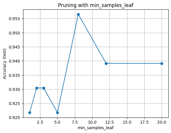
Hint for interpretation: very small leaves may overfit while very large leaves may underfit.

---

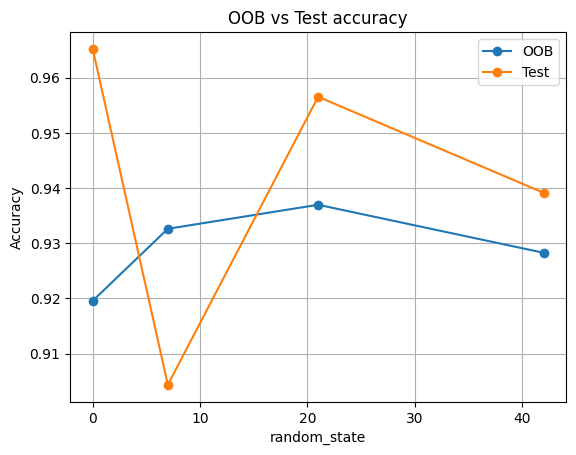
Q3

seeds = [0, 7, 21, 42]
rows_oob = []

for s in seeds:
    X_tr, X_te, y_tr, y_te = train_test_split(X, y, test_size=0.2, random_state=s, stratify=y)
    rf = RandomForestClassifier(
        n_estimators=300, max_features="sqrt", min_samples_leaf=3,
        oob_score=True, random_state=s
    ).fit(X_tr, y_tr)
    acc_test = accuracy_score(y_te, rf.predict(X_te))
    rows_oob.append({"seed": s, "OOB": rf.oob_score_, "TestAcc": acc_test})

pd.DataFrame(rows_oob).round(3)

	seed	OOB	TestAcc
0	0	0.920	0.965
1	7	0.933	0.904
2	21	0.937	0.957
3	42	0.928	0.939

df_oob = pd.DataFrame(rows_oob)
plt.plot(df_oob["seed"], df_oob["OOB"], "o-", label="OOB")
plt.plot(df_oob["seed"], df_oob["TestAcc"], "o-", label="Test")
plt.xlabel("random_state")
plt.ylabel("Accuracy")
plt.title("OOB vs Test accuracy")
plt.grid(True)
plt.legend()
plt.show()

small_tree = DecisionTreeClassifier(max_depth=2, random_state=0).fit(X_train, y_train)

plt.figure(figsize=(7,5))
plot_tree(small_tree, feature_names=feat_names, class_names=["non_toxic","toxic"], filled=True)
plt.title("Small Decision Tree (max_depth=2)")
plt.show()

# Extract split rules programmatically for the top two levels
feat_idx = small_tree.tree_.feature
thresh = small_tree.tree_.threshold
left = small_tree.tree_.children_left
right = small_tree.tree_.children_right

def node_rule(node_id):
    f = feat_idx[node_id]
    t = thresh[node_id]
    return f"{feat_names[f]} <= {t:.3f} ?"

print("Root rule:", node_rule(0))
print("Left child rule:", node_rule(left[0]) if left[0] != -1 else "Left child is a leaf")
print("Right child rule:", node_rule(right[0]) if right[0] != -1 else "Right child is a leaf")

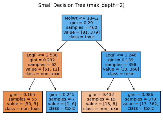
Root rule: MolWt <= 134.200 ?
Left child rule: LogP <= 2.538 ?
Right child rule: LogP <= 1.248 ?

Expect OOB to track test accuracy closely. Small differences are normal.

---

Q4

Compare built-in importance to permutation importance for a random forest regressor.

rf_imp = RandomForestRegressor(
    n_estimators=400, min_samples_leaf=3, max_features="sqrt",
    random_state=0
).fit(Xr_train, yr_train)

# Built-in importance
imp_series = pd.Series(rf_imp.feature_importances_, index=Xr_train.columns).sort_values()

# Permutation importance on test
perm_r = permutation_importance(
    rf_imp, Xr_test, yr_test, scoring="r2", n_repeats=20, random_state=0
)
perm_series = pd.Series(perm_r.importances_mean, index=Xr_train.columns).sort_values()

# Plots
imp_series.plot(kind="barh")
plt.title("Random Forest feature_importances_ (regression)")
plt.show()

perm_series.plot(kind="barh")
plt.title("Permutation importance on test (regression)")
plt.show()

pd.DataFrame({"Built_in": imp_series, "Permutation": perm_series})

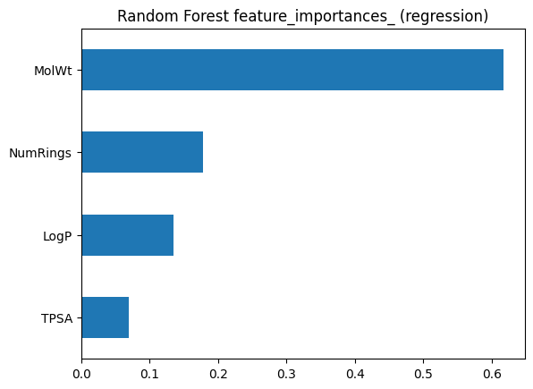
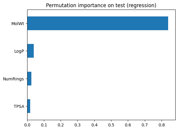
	Built_in	Permutation
LogP	0.135308	0.039454
MolWt	0.617161	0.839382
NumRings	0.177916	0.025688
TPSA	0.069615	0.017808

Look for agreement on the top features. Disagreements can signal correlation or overfitting in the training trees.

---

Q5

url = "https://raw.githubusercontent.com/zzhenglab/ai4chem/main/book/_data/C_H_oxidation_dataset.csv"
df_raw = pd.read_csv(url)
desc = df_raw["SMILES"].apply(calc_descriptors)
df = pd.concat([df_raw, desc], axis=1)

# 2) Build classification frame and clean
label_map = {"toxic": 1, "non_toxic": 0}
df_clf = df[["MolWt", "LogP", "TPSA", "NumRings", "Toxicity"]].dropna()
df_clf = df_clf[df_clf["Toxicity"].str.lower().isin(label_map.keys())]

X = df_clf[["MolWt", "LogP", "TPSA", "NumRings"]]
y = df_clf["Toxicity"].str.lower().map(label_map).astype(int)

# Guard against degenerate stratify cases
assert y.nunique() == 2, "Need both classes for stratified split"

X_train, X_test, y_train, y_test = train_test_split(
    X, y, test_size=0.2, random_state=15, stratify=y
)

# 3) CV setup and grid
cv = KFold(n_splits=5, shuffle=True, random_state=0)
param_grid = {
    "n_estimators": [200, 400],
    "max_depth": [None, 6, 10],
    "min_samples_leaf": [1, 2, 3, 5],
    "max_features": ["sqrt", 0.8],
}

rf_base = RandomForestClassifier(random_state=0)

grid = GridSearchCV(
    rf_base,
    param_grid=param_grid,
    scoring="roc_auc",
    cv=cv,
    refit=True,
    return_train_score=False,
)

# 4) Fit and report
grid.fit(X_train, y_train)
print("Best params:", grid.best_params_)
print(f"Best CV AUC: {grid.best_score_:.3f}")

rf_best = grid.best_estimator_

y_hat = rf_best.predict(X_test)
y_proba = rf_best.predict_proba(X_test)[:, 1]
print(f"Test Accuracy: {accuracy_score(y_test, y_hat):.3f}")
print(f"Test AUC: {roc_auc_score(y_test, y_proba):.3f}")

# 5) ROC curve
fpr, tpr, thr = roc_curve(y_test, y_proba)
plt.plot(fpr, tpr, lw=2)
plt.plot([0, 1], [0, 1], "k--")
plt.xlabel("FPR")
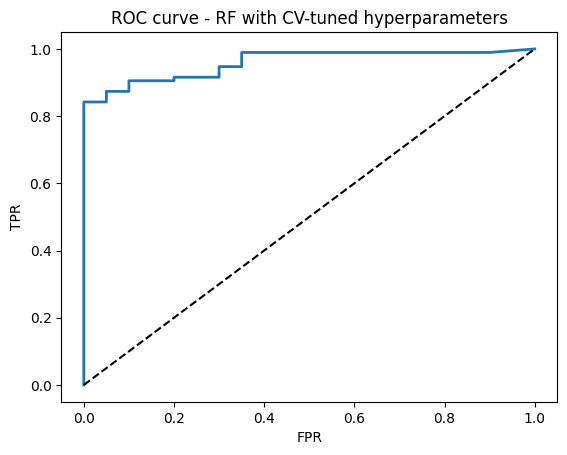
plt.ylabel("TPR")
plt.title("ROC curve - RF with CV-tuned hyperparameters")
plt.show()

Best params: {'max_depth': 6, 'max_features': 'sqrt', 'min_samples_leaf': 2, 'n_estimators': 200}
Best CV AUC: 0.980
Test Accuracy: 0.922
Test AUC: 0.959